Turbulence Modelling in CFD — Theory, Numerics and Industrial Applications
Understand turbulence physics, Reynolds averaging, turbulent transport, RANS, LES, DNS, turbulence closures, wall modelling, y+, numerical schemes, OpenFOAM implementation, validation, and industrial CFD applications.
1. Introduction: Why Turbulence Matters
Imagine water flowing through a narrow pipe.
At a sufficiently low flow rate, the water can move in smooth, orderly layers. Increase the flow rate, and the motion may become irregular. Small disturbances grow, vortices form, and velocity and pressure fluctuate continuously.
Now imagine air flowing over an aircraft wing, water passing through a hydraulic turbine, coolant moving through a heat exchanger, or air circulating around a vehicle.
In these applications, the flow may contain a wide range of interacting motions, from large swirling structures to very small fluctuations.
This is turbulence.
Turbulence is one of the most important and challenging topics in computational fluid dynamics (CFD). It influences:
- Aerodynamic drag and lift
- Pressure losses in pipes and ducts
- Heat transfer in cooling systems
- Mixing in chemical reactors
- Flow separation around vehicles
- Noise generation
- Combustion and pollutant transport
- Cavitation and unsteady loads in hydraulic machinery
- Flow-induced vibration
- Particle transport in fluid-solid systems
For many industrial applications, the difference between a useful CFD prediction and a misleading one depends heavily on how turbulence is represented.
A solver can calculate velocity and pressure fields, but a practical simulation must also account for the effects of turbulent fluctuations that cannot be fully resolved on an affordable computational mesh.
This is where turbulence modelling becomes essential.
At a glance, turbulence is not a single phenomenon but a family of interacting flow structures: large eddies, shear layers, recirculation regions, and tiny dissipative motions all coexist. The challenge in CFD is not to model turbulence as a mysterious defect, but to represent its net effect on the mean flow, heat transfer, and pressure loss in a way that is consistent with the engineering question.
The objective of this module is to develop a physical understanding first, then connect that understanding to mathematical models, numerical methods, mesh requirements, and practical simulation workflows.
By the end, you should be able to:
- Explain the physical characteristics of turbulent flow.
- Understand the Reynolds number and its limitations as a transition indicator.
- Derive the basic idea behind Reynolds-averaged Navier–Stokes equations.
- Explain Reynolds stresses, turbulent kinetic energy, and eddy viscosity.
- Distinguish RANS, URANS, LES, hybrid methods, and DNS.
- Compare common models such as -, - SST, and Reynolds stress models.
- Understand wall functions, near-wall resolution, and .
- Recognize the effects of mesh quality, discretization, time step, and numerical diffusion.
- Configure and evaluate a turbulence model in OpenFOAM.
- Develop a systematic verification and validation strategy.
2. What Is Turbulence?
Turbulence is an irregular, three-dimensional and time-dependent state of fluid motion characterized by fluctuating velocities and interacting flow structures.
Unlike a simple smooth flow, turbulent motion contains a broad range of spatial and temporal scales.
Consider smoke released into still air.
At first, the smoke may form a relatively smooth column. Farther downstream, the column can develop swirls, bends, and smaller irregular structures. These motions interact and transport momentum, heat, and mass.
The resulting flow is not random in the sense that physics no longer applies. It still obeys conservation of mass, momentum, and energy. However, its instantaneous structure can be extremely complex.
2.1 The main characteristics of turbulence
Irregular fluctuations
Velocity and pressure change with time and position. A point in a turbulent flow can experience rapid changes in its local velocity.
Three-dimensional motion
Turbulent flows generally contain interacting motions in all three spatial directions, even when the mean flow appears primarily two-dimensional.
Mixing
Turbulent fluctuations transport momentum, heat, and species between neighbouring regions much more effectively than molecular diffusion alone in many high-Reynolds-number flows.
Vorticity
Turbulent flows often contain vortices and regions of concentrated rotation. These structures stretch, tilt, interact, and break down into smaller scales.
A wide range of scales
Large turbulent structures may be comparable to the geometry of the flow, while the smallest dynamically important structures can be many orders of magnitude smaller.
Dissipation
Viscosity converts kinetic energy associated with small-scale motion into internal energy. This process is called viscous dissipation.
2.2 Is turbulence always chaotic everywhere?
No. A turbulent flow may contain regions with different behaviours.
For example, flow around a vehicle can include:
- A turbulent boundary layer on the body
- A separated shear layer behind a sharp edge
- Large recirculating structures in the wake
- Regions with relatively weak velocity fluctuations
- Areas where turbulence decays downstream
The engineering challenge is to predict the important effects of these structures, not merely to label the entire flow as turbulent.
2.3 Physical example: mixing coffee
When you stir coffee, a spoon creates large-scale motion. The liquid then develops smaller swirls and irregular fluctuations.
These motions transport heat and dissolved substances more effectively than molecular diffusion alone.
The same physical principle applies to:
- Mixing fuel and air in a combustion chamber
- Mixing reactants in a chemical reactor
- Distributing coolant temperature in a heat exchanger
- Mixing hot and cold air in a ventilation system
Turbulence is therefore not only a source of computational difficulty. It is also a mechanism engineers deliberately use to improve transport and mixing.
2.4 Visualizing turbulent flow
The following NASA resource shows how smoke and other flow-visualization methods can reveal vortices and separated flow in experiments.
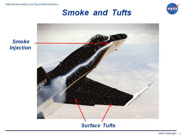
Image source: NASA Glenn Research Center, Smoke and Tuft Flow Visualization. Use the source page if the embedded image does not load.
3. Laminar Flow, Transition and Turbulent Flow
Before choosing a turbulence model, it is important to understand the difference between laminar and turbulent motion.
3.1 Laminar flow
In laminar flow, fluid motion is relatively orderly, and neighbouring layers exchange momentum mainly through molecular transport.
For fully developed laminar flow in a straight circular pipe, the velocity profile is parabolic:
- The velocity is zero at the wall because of the no-slip condition.
- The velocity increases toward the centreline.
- The centreline velocity is twice the bulk mean velocity for the ideal fully developed circular-pipe solution.
Laminar flow can still have strong velocity gradients, heat transfer, and viscous forces. It is not necessarily slow or unimportant.
3.2 Transitional flow
Transition is the process through which disturbances in a laminar flow grow and the flow develops turbulent fluctuations.
Transition depends on more than Reynolds number. Influencing factors include:
- Disturbance levels at the inlet
- Surface roughness
- Pressure gradients
- Geometry
- Free-stream turbulence
- Acoustic disturbances
- Wall temperature and fluid properties
For some applications, transition itself is the primary engineering concern.
Examples include aircraft wings, turbine blades, wind-turbine blades, and low-drag surfaces.
A fully turbulent model should not automatically be applied when the objective is to predict the location of laminar-to-turbulent transition.
3.3 Turbulent flow
In turbulent flow, velocity fluctuations generate additional transport of momentum and other quantities.
The mean velocity profile is often fuller than its laminar counterpart. In a turbulent pipe, for example, the mean velocity remains relatively high across much of the cross-section and then changes more sharply near the wall.
This behaviour is associated with stronger mixing across the flow.
The wall region remains especially important because it controls friction, near-wall transport, and often a large part of the heat transfer.
3.4 Visual comparison of boundary-layer velocity profiles
A boundary layer develops when fluid flows over a solid surface. The no-slip condition forces the fluid velocity to approach zero at the wall.
The turbulent profile shown below is a standard educational comparison from a public-domain source, intended to illustrate the qualitative difference between laminar and turbulent momentum transport.

The exact profile depends on geometry, Reynolds number, pressure gradient, roughness, and other flow conditions. The key lesson is that turbulence redistributes momentum and therefore affects skin friction, separation, and heat transfer.
For a reference illustration of boundary-layer profiles, see Turbulent and Laminar Boundary Layer Profiles on Wikimedia Commons.

4. Reynolds Number: A Useful Indicator, Not a Universal Transition Switch
The Reynolds number compares inertial forces with viscous forces.
where:
- : density, kg/m³
- : characteristic velocity, m/s
- : characteristic length, m
- : dynamic viscosity, Pa·s
- : kinematic viscosity, m²/s
A high Reynolds number generally means that inertial effects are large relative to molecular viscous effects at the selected scale.
This often permits strong flow instabilities and a broad range of turbulent motions. However, Reynolds number alone does not determine whether every flow will be turbulent.
4.1 Example: water flowing through a pipe
Assume:
- Mean velocity m/s
- Pipe diameter m
- Kinematic viscosity m²/s
Then:
This Reynolds number is well above the range where a smooth, straight circular pipe normally remains fully laminar under ordinary conditions.
A turbulent-flow treatment would therefore be a reasonable starting point for many engineering calculations, subject to the actual inlet and pipe conditions.
4.2 Typical pipe-flow interpretation
For fully developed flow in a smooth circular pipe, engineers often use the following approximate guide:
| Pipe Reynolds number | Typical interpretation |
|---|---|
| Usually laminar | |
| Transitional range | |
| Usually turbulent |
These values are not universal transition criteria for external flows, complex ducts, rotating machinery, or flows with strong disturbances.
Important: Do not use pipe-flow transition thresholds as a universal rule for every CFD geometry.
5. Why Turbulence Is Difficult to Resolve Numerically
The incompressible Navier–Stokes equations are:
These equations describe conservation of mass and momentum for an incompressible Newtonian fluid with constant density and viscosity, under the assumptions stated.
The nonlinear convection term,
allows different flow structures to interact.
A large swirling motion can stretch smaller vortices. Smaller vortices interact and produce finer structures. This process continues toward scales where viscosity dissipates the kinetic energy.
In turbulent flows, the relevant scales may span a very large range.
A computational simulation must decide which scales to resolve directly and which to represent using a model.
Resolving every dynamically relevant scale for a high-Reynolds-number industrial flow can require an enormous number of cells and very small time steps.
That is why industrial CFD generally uses turbulence modelling rather than resolving every turbulent motion directly.
6. Turbulent Energy Cascade
Turbulent motion contains kinetic energy across a range of length scales.
A simplified explanation is:
- Large-scale motions receive energy from the mean flow or the external forcing.
- These motions interact and transfer energy to smaller scales.
- Smaller structures transfer energy to even smaller scales.
- Viscosity eventually dissipates the kinetic energy into internal energy.
This process is known as the turbulent energy cascade.
The largest structures are often strongly influenced by the geometry. The smallest scales are more directly controlled by viscosity.
This distinction helps explain the different turbulence-modelling strategies.
- RANS models the net effects of turbulent fluctuations.
- LES resolves larger turbulent motions and models smaller subgrid motions.
- DNS resolves the full range of dynamically relevant turbulent scales without a turbulence closure model.
6.1 Schematic energy spectrum
A useful mental picture is that turbulent kinetic energy is injected at large scales, transferred through the inertial range, and finally dissipated at the smallest scales by viscosity.

Image source: Wikimedia Commons, public-domain educational schematic.
In classical homogeneous, isotropic turbulence, the inertial-range energy spectrum is often associated with Kolmogorov’s power law under appropriate assumptions. Real industrial flows can depart from this idealized behaviour because of walls, anisotropy, strong mean shear, compressibility, and other effects.
7. The Fundamental Idea of Turbulence Modelling
The central difficulty is not that the Navier–Stokes equations stop working in turbulent flow.
The difficulty is that directly resolving all turbulent scales is too expensive for many engineering applications.
Turbulence modelling approximates the effects of unresolved turbulent motions on the quantities we want to predict.
Imagine trying to describe the movement of a crowded street.
You could track every person individually, or you could model the average flow of people through different sections of the street.
The first approach contains more detailed information but is much more expensive. The second approach can answer many practical questions more efficiently, but it does not predict every individual’s path.
The same idea applies to turbulence modelling, although the mathematical details are much more complex.
There are several main strategies:
- RANS: Model the influence of turbulent fluctuations on the mean flow.
- URANS: Retain time dependence in a RANS formulation to represent unsteady large-scale behaviour of the modelled flow.
- LES: Resolve larger turbulent motions and model smaller motions below the filter scale.
- Hybrid RANS–LES: Use RANS modelling in selected regions and scale-resolving treatment in others.
- DNS: Resolve all dynamically relevant turbulent scales directly without a turbulence closure model.
No single method is best for every engineering problem.
8. Reynolds Decomposition: Separating Mean Flow and Fluctuations
In Reynolds-averaged modelling, an instantaneous velocity is decomposed into a mean component and a fluctuating component:
where:
- : instantaneous velocity component, m/s
- : mean velocity component, m/s
- : fluctuating velocity component, m/s
For a suitable averaging procedure:
The mean is often a time average for statistically stationary flow, but averaging may instead be ensemble-based or defined in another suitable way.
For a stationary flow with an adequate averaging interval:
where is the averaging interval.
The choice of averaging interval matters. If it is too short, the estimated mean may still contain substantial unsteady variation.
8.1 Example: a velocity signal
Suppose a velocity probe records the following illustrative values:
| Time sample | Instantaneous velocity |
|---|---|
| 1 | 8.8 m/s |
| 2 | 10.5 m/s |
| 3 | 9.2 m/s |
| 4 | 11.0 m/s |
| 5 | 10.5 m/s |
The average is:
The instantaneous values fluctuate around the average.
A RANS calculation seeks the mean-flow field and models the statistical effects of the fluctuations. It does not attempt to reproduce this particular five-sample sequence.
The values above are an arithmetic example, not experimental data.
9. The Reynolds-Averaged Navier–Stokes Equations
Apply Reynolds decomposition to the governing equations and average them over time or an appropriate statistical ensemble.
The resulting equations describe the mean flow.
For constant-density incompressible flow:
The averaged momentum equation can be written as:
Repeated indices imply summation over spatial directions.
The new term,
represents the influence of velocity fluctuations on the mean momentum balance.
This is the essential challenge of Reynolds-averaged turbulence modelling.
The averaging operation introduces additional unknown correlations. The equations are no longer closed by the mean velocity and pressure alone.
This is called the closure problem.
9.1 Reynolds stresses
The tensor
is commonly called the Reynolds-stress covariance tensor. The associated Reynolds stress in the momentum equation is often written as:
under this sign convention.
The individual components describe how velocity fluctuations are correlated.
For example:
measures the correlation between streamwise and wall-normal velocity fluctuations.
This correlation is especially important in a wall-bounded shear flow because it contributes to the transport of streamwise momentum in the wall-normal direction.
9.2 Physical meaning of Reynolds stresses
Imagine a turbulent boundary layer over a flat plate.
Some fluid parcels move away from the wall carrying relatively high streamwise momentum. Others move toward the wall carrying lower streamwise momentum.
These correlated motions produce a net turbulent transport of streamwise momentum.
The Reynolds stresses represent the mean influence of such fluctuations.
They are not ordinary molecular viscosity. They are additional terms arising from the averaging of nonlinear fluid motion.
9.3 Why turbulence models are needed
The mean-flow equations contain Reynolds stresses that must be estimated.
Different turbulence models use different approximations to obtain them.
Examples include:
- Algebraic eddy-viscosity models
- One-equation models
- Two-equation models
- Nonlinear eddy-viscosity models
- Reynolds stress transport models
The choice determines how much information the model solves for and how it represents anisotropy, rotation, separation, and turbulent transport.
For the theoretical derivation and formulation of RANS models, see the OpenFOAM RAS documentation.
10. Turbulent Kinetic Energy
Turbulent kinetic energy, commonly denoted by , measures the kinetic energy associated with velocity fluctuations per unit mass.
In three dimensions:
Its unit is:
Turbulent kinetic energy is not the same as the mean kinetic energy of the flow.
A flow can have a high mean velocity but relatively weak turbulence, or a lower mean velocity with strong fluctuations.
The distinction matters when estimating mixing, turbulent transport, and unsteady loads.
10.1 Example: two cooling ducts
Consider two ducts with the same mean velocity.
- Duct A has a smooth, uniform inlet profile and relatively low fluctuations.
- Duct B receives flow from a sharp bend and has a strongly disturbed velocity field.
Even though the mean velocities may be similar, the turbulence levels and downstream mixing may differ substantially.
A turbulence model must represent these differences sufficiently well for the engineering objective.
10.2 Turbulence intensity
A commonly used measure of turbulence intensity is:
where:
- : root-mean-square velocity fluctuation in a selected direction, m/s
- : representative mean velocity, m/s
For approximately isotropic turbulence, one sometimes estimates:
and therefore:
This relationship relies on the assumption that the three fluctuation components have similar variances. It is not generally exact for strongly anisotropic flows.
Turbulence intensity is frequently used to help specify inlet turbulence conditions, but it does not fully characterize the turbulence structure.
11. The Eddy-Viscosity Concept
A common approach to modelling Reynolds stresses is the Boussinesq eddy-viscosity hypothesis.
For incompressible flow, its simplified form is:
where:
and:
- : turbulent kinematic viscosity, m²/s
- : turbulent kinetic energy, m²/s²
- : Kronecker delta
- : mean strain-rate tensor, 1/s
For a compressible or variable-density formulation, the exact equations and averaging conventions differ.
11.1 What does eddy viscosity mean?
Molecular viscosity describes momentum transport due to molecular processes.
Eddy viscosity is a modelling quantity used to represent the additional momentum transport caused by turbulent fluctuations.
It is not a separate physical fluid property. It is calculated from the turbulence model and the local flow conditions.
The effective momentum transport can be much larger than molecular transport in strongly turbulent regions.
11.2 An analogy
Imagine a crowd moving through a corridor.
People walking across the corridor carry their streamwise momentum with them. The resulting transport may be much stronger than if people moved only in perfectly ordered parallel lines.
Eddy viscosity provides a simplified way to represent the additional mixing in the mean momentum equations.
However, turbulence is not literally a fluid with a higher molecular viscosity.
11.3 Limitations of the eddy-viscosity hypothesis
A simple eddy-viscosity model assumes that the anisotropic Reynolds stresses are related to the mean strain rate in a specified way.
This can work well for many engineering flows.
However, turbulence can become strongly anisotropic or respond to physical effects that are not represented well by a simple linear relation.
Examples include:
- Strong streamline curvature
- Rapid rotation
- Swirling flows
- Secondary flows in non-circular ducts
- Strong separation
- Some flows with substantial stress anisotropy
This motivates more advanced turbulence closures.
12. The Main Turbulence-Modelling Approaches
12.1 RANS — Reynolds-Averaged Navier–Stokes
RANS solves equations for mean flow quantities and models the statistical effect of turbulent fluctuations.
The turbulence model supplies the additional relationships needed to close the equations.
Advantages
- Relatively affordable computational cost
- Widely used in industrial design
- Suitable for many engineering mean-flow predictions
- Can be used in steady-state or transient formulations
Limitations
- Does not resolve the full instantaneous turbulent structure
- Accuracy depends on the closure model
- May struggle with complex separation, strong anisotropy, and certain unsteady flows
RANS is often the first modelling approach to consider for industrial design studies.
12.2 URANS — Unsteady RANS
URANS retains the time-dependent terms in the RANS equations.
It can represent time-varying mean flow and some large-scale periodic behaviour, but its solution is still based on a RANS turbulence closure.
A transient URANS calculation does not automatically resolve all turbulent eddies.
This distinction is important when interpreting wake structures, vortex shedding, and transient aerodynamic loads.
12.3 LES — Large Eddy Simulation
LES resolves larger turbulent structures while modelling the effects of smaller, unresolved motions.
A spatial filter separates the resolved field from the subgrid-scale field.
The large structures are directly represented by the numerical solution, while a subgrid-scale model accounts for the influence of motions smaller than the filter scale.
Advantages
- Provides time-dependent information about large turbulent structures
- Can represent unsteady separated flows more naturally than many RANS approaches
- Useful for mixing, wake dynamics, and fundamental turbulence research
Limitations
- Usually more computationally expensive than RANS
- Requires three-dimensional, transient calculations for conventional LES
- Needs sufficient spatial and temporal resolution
- Near-wall resolution can become particularly expensive at high Reynolds numbers
12.4 Hybrid RANS–LES methods
Hybrid methods combine RANS and LES-like treatment.
A common strategy is to use RANS modelling near walls and resolve larger turbulent structures in separated regions.
Examples include detached-eddy simulation (DES) and related scale-resolving approaches.
These methods can provide a practical compromise for complex industrial flows, but their performance depends on grid design, model formulation, and the ability of the mesh to support resolved turbulent structures.
12.5 DNS — Direct Numerical Simulation
DNS solves the governing fluid equations without a turbulence closure model for the dynamically relevant turbulent scales.
The computational mesh and time step must be fine enough to resolve the smallest relevant motions.
DNS is extremely expensive at high Reynolds numbers, especially in wall-bounded flows.
It is therefore primarily used for fundamental research, model development, and high-quality reference data rather than routine industrial design.
12.6 Comparison of modelling approaches
| Method | What is resolved? | What is modelled? | Typical role |
|---|---|---|---|
| RANS | Mean flow | Turbulent fluctuation effects | Industrial design and parameter studies |
| URANS | Time-dependent mean flow | Turbulence closure effects | Some unsteady engineering flows |
| LES | Large turbulent structures | Subgrid-scale effects | Detailed transient turbulence |
| Hybrid RANS–LES | Mean and selected resolved structures | Unresolved turbulence, depending on region | Complex separated flows |
| DNS | All dynamically relevant scales | No turbulence closure | Fundamental research and reference data |
The computational cost generally increases from RANS toward DNS for comparable high-Reynolds-number engineering problems, but the exact cost and predictive value depend on the geometry, physical model, numerical method, and required output.
The NASA Turbulence Modeling Resource provides model documentation, verification cases, and reference data.
13. Understanding Common RANS Turbulence Models
RANS is a modelling framework, not one single turbulence model.
Different closures use different assumptions to estimate turbulent stresses and transport.
13.1 Spalart–Allmaras
Spalart–Allmaras is a one-equation eddy-viscosity model.
It solves a transport equation for a turbulence-related variable from which turbulent viscosity is constructed.
It is widely associated with aerodynamic applications, including external flows around aircraft and other streamlined bodies.
Potential strengths
- Relatively economical
- Often useful for attached aerodynamic boundary layers
- Established in many aerospace CFD workflows
Potential limitations
- May be less suitable for flows requiring a detailed representation of turbulence anisotropy
- Separation and strongly complex flows require careful assessment
- Model performance depends on the flow class and implementation
13.2 Standard -
The standard - model solves transport equations for:
- : turbulent kinetic energy, m²/s²
- : turbulent kinetic-energy dissipation rate, m²/s³
A characteristic turbulent-viscosity relation is:
where is a model coefficient.
The model is widely used for industrial internal flows, mixing, and many general engineering applications.
It is often robust and economical, especially when used with a compatible wall-function approach.
However, the standard formulation may have limitations in strong adverse pressure gradients, separation, and certain rotation- or curvature-dominated flows.
13.3 Standard -
The standard - model solves transport equations for:
- : turbulent kinetic energy
- : specific dissipation rate, s⁻¹
A characteristic eddy-viscosity relation is:
The exact relation and any limiting operations depend on the model formulation.
The model is often attractive for near-wall flows because the -based formulation can be integrated close to the wall without relying on the same high-Reynolds-number wall-function strategy used by some - implementations.
However, standard - models can be sensitive to the specification of in the free stream.
13.4 - SST
The shear-stress transport (SST) model combines features of - and --type formulations using blending functions.
Its purpose is to improve behaviour across the near-wall and outer-flow regions and to limit the turbulent shear stress in a manner useful for adverse-pressure-gradient flows.
SST is widely used for:
- Aerodynamic bodies
- Diffusers
- Turbomachinery passages
- Separated boundary layers
- External flows with possible separation
It is often a sensible starting point when separation and near-wall behaviour matter.
It is not guaranteed to predict every separated flow accurately. Results should be checked against suitable reference data and mesh studies.
13.5 Reynolds stress models
A Reynolds stress transport model solves transport equations for individual Reynolds-stress components rather than relying entirely on a simple scalar eddy-viscosity relation.
These models can represent stress anisotropy more directly.
They may be useful for:
- Strongly swirling flows
- Complex secondary flows
- Rotation-dominated systems
- Flows where Reynolds-stress anisotropy is important
The additional equations increase computational cost and can make convergence more challenging.
13.6 Transition models
Transition models attempt to predict the development of turbulence from a laminar state.
They are important when laminar-to-turbulent transition materially affects the result.
Examples include transition-sensitive formulations used with selected RANS models.
A fully turbulent RANS model may produce reasonable results for a fully turbulent flow but cannot necessarily predict the correct transition location.
13.7 How should an engineer select a model?
Do not select a turbulence model based only on popularity.
Ask:
- Is the flow attached or separated?
- Is the boundary layer important?
- Are strong pressure gradients present?
- Is rotation or swirl important?
- Is transition a design concern?
- Are instantaneous turbulent structures required?
- What reference data are available?
- What is the computational budget?
- Can the chosen model’s mesh and wall-treatment requirements be satisfied?
A practical approach is to start with a well-supported baseline model, validate it for the relevant flow class, and compare alternatives when model uncertainty matters.
14. Wall-Bounded Turbulence and the Near-Wall Region
Many engineering flows are strongly influenced by solid walls.
Examples include:
- Flow inside a pipe
- Air over an aircraft wing
- Coolant flowing through a cold plate
- Flow through a hydraulic turbine
- Air moving around a car
- Flow through a heat exchanger
The region close to the wall is called the boundary layer.
At a stationary, impermeable wall, the no-slip condition requires the fluid velocity relative to the wall to be zero.
The velocity then increases away from the wall until it approaches the outer-flow velocity.
In turbulent boundary layers, several characteristic regions are often distinguished.
14.1 Viscous sublayer
Very close to the wall, molecular viscosity strongly influences momentum transport.
In an idealized smooth-wall turbulent boundary layer, the dimensionless mean velocity is approximately linear:
over the viscous-dominated region.
14.2 Buffer layer
The buffer region is where viscous and turbulent effects are both important.
It connects the viscous-dominated near-wall behaviour with the outer turbulent region.
14.3 Logarithmic region
For suitable high-Reynolds-number, approximately equilibrium wall flows, the mean velocity can follow a logarithmic law over part of the inner region:
where is the von Kármán constant and depends on the flow and conventions used.
This is an approximate law, not a universal exact solution for all wall-bounded flows.
14.4 Why the near-wall region matters
Near-wall predictions influence:
- Skin-friction drag
- Wall shear stress
- Pressure loss
- Heat transfer
- Separation
- Component loads
- Turbulent production
A simulation can have a very large number of cells overall but still predict wall shear or heat transfer poorly if the near-wall mesh and turbulence treatment are inconsistent.
15. What Is ?
The dimensionless wall distance is defined as:
where:
- : friction velocity, m/s
- : wall-normal distance from the wall to the first cell-centre location, m
- : kinematic viscosity, m²/s
The friction velocity is:
where is the wall shear stress magnitude.
The quantity indicates where the first computational cell lies relative to the characteristic near-wall viscous scale.
15.1 Why is useful?
The value helps determine whether the near-wall mesh is compatible with the selected wall treatment.
Two common strategies are:
Wall-resolved modelling
The mesh resolves the near-wall viscous region. For many wall-resolved SST applications, a target near is a common starting point.
Wall-function modelling
The near-wall region is treated using a wall-function formulation. Depending on the model and implementation, the first cell is often placed in the log-layer range, rather than inside the viscous sublayer.
The correct range is model-specific. Do not assume that one universal target applies to all turbulence models or wall functions.
15.2 Example: estimating first-cell height
Suppose:
- Estimated friction velocity: m/s
- Air kinematic viscosity: m²/s
- Target:
Rearranging:
The estimated wall-normal distance from the wall to the first cell centre is:
This is only a first estimate. The actual depends on the local wall shear stress, which may change as the solution develops.
For a cell-centred finite-volume mesh, distinguish the first-cell-centre distance from the full cell height when applying the estimate.
15.3 A practical near-wall checklist
- Choose the turbulence model and wall treatment first.
- Estimate the first-cell height using representative operating conditions.
- Add enough layers to resolve the relevant boundary-layer thickness.
- Use suitable layer growth and total thickness.
- Check the resulting distribution after solving.
- Inspect wall shear, pressure drop, and heat transfer for mesh sensitivity.
- Avoid interpreting without considering the model’s intended near-wall formulation.
For OpenFOAM-specific mesh guidance, consult the turbulence modelling documentation.
16. Turbulence Numerics: How the Equations Are Solved
Turbulence modelling is only one part of the simulation.
The equations must also be discretized on a computational mesh and solved numerically.
Three important sources of error are:
- Physical-model error
- Spatial and temporal discretization error
- Iterative or algebraic solution error
A turbulence model cannot compensate for every numerical deficiency.
16.1 Spatial discretization
CFD converts differential equations into algebraic equations associated with computational cells or other discrete locations.
For a finite-volume method, a conservation equation is integrated over each control volume.
The resulting balance includes fluxes across cell faces and source terms within the cell.
The mesh must resolve the important mean-flow gradients and, in LES, the large turbulent structures intended to be resolved.
16.2 Numerical diffusion
Numerical diffusion is artificial smoothing introduced by the discretization.
It can smear velocity gradients, weaken shear layers, and reduce the strength of resolved vortices.
In RANS, excessive numerical diffusion can alter the mean flow and the turbulence production predicted by the model.
In LES, it can suppress resolved turbulent fluctuations and undermine the purpose of scale-resolving simulation.
A bounded, stable numerical scheme is important, but excessive numerical dissipation should not be ignored.
16.3 Gradient and convection schemes
The calculated velocity gradient affects turbulence production in many models.
Poor mesh quality or inaccurate gradient reconstruction can therefore affect:
- Turbulent kinetic energy
- Eddy viscosity
- Reynolds stresses
- Separation behaviour
- Numerical stability
Convection schemes must balance accuracy, boundedness, and stability.
Higher-order schemes can improve accuracy when the mesh and solution support them, but they may require more careful numerical control.
16.4 Pressure-velocity coupling
For incompressible flow, pressure and velocity are coupled through the continuity constraint.
Algorithms such as SIMPLE and PISO are widely used in finite-volume CFD.
The choice depends on the solver, steady or transient formulation, and implementation.
Turbulence equations are solved as part of the coupled numerical process, and their stability may depend on the velocity and pressure solution.
16.5 Steady-state versus transient calculations
A steady RANS calculation seeks a stationary mean-flow solution.
A transient RANS calculation retains time dependence, but the turbulence closure remains based on averaged or modelled quantities.
LES requires a time-dependent solution because its purpose includes resolving turbulent structures that evolve in time.
For LES, the time step must be sufficiently small to capture the resolved dynamics, and the mesh must be adequate for the intended resolved scales.
A transient solver does not automatically mean that turbulence is being resolved.
17. Turbulence Production and Dissipation
Turbulence models often represent a balance between production, transport, and dissipation of turbulent kinetic energy.
A simplified conceptual balance is:
This is a conceptual equation rather than a complete transport equation.
17.1 Production
Turbulent kinetic energy is produced when the turbulent stresses interact with mean velocity gradients.
In a common incompressible RANS formulation, the production term is related to:
The sign and exact form depend on the adopted stress and production conventions.
In a simple shear flow, mean velocity gradients can transfer energy from the mean motion into turbulent fluctuations.
17.2 Dissipation
Dissipation represents the conversion of turbulent kinetic energy into internal energy by viscous action at small scales.
In the - model, represents the turbulent kinetic-energy dissipation rate.
Its unit is:
17.3 Transport
Turbulent kinetic energy is also transported by:
- Mean advection
- Turbulent diffusion
- Molecular diffusion
- Pressure-related transport, depending on the formulation
The balance differs across geometries and flow regimes.
For example, a wake behind a bluff body can have strong turbulence production near the separated shear layers, followed by downstream transport and decay.
This is why turbulence-model performance should be assessed against the actual flow class rather than assumed to be uniform across all applications.
18. Turbulence Boundary Conditions
A turbulence model needs suitable initial and boundary values for its turbulence variables.
Common inputs include turbulence intensity, turbulent length scale, turbulent kinetic energy, dissipation rate, and specific dissipation rate.
The required fields depend on the model.
18.1 Turbulence intensity
For an approximately isotropic inlet turbulence assumption:
where:
- : representative inlet velocity, m/s
- : turbulence intensity as a fraction, dimensionless
For example, an inlet velocity of 10 m/s and turbulence intensity of 5% gives:
This is a model-based estimate, not a direct measurement of the complete turbulence structure.
18.2 Turbulence length scale
A turbulence length scale represents the characteristic size of energy-containing turbulent structures.
For internal flows, engineers sometimes estimate it using a fraction of a characteristic hydraulic diameter. Such estimates are practical approximations, not universal physical laws.
The choice should reflect the geometry, upstream conditions, and available measurements.
18.3 Estimating and
For some commonly used two-equation model formulations, approximate inlet values can be estimated from , a turbulence length scale , and model coefficients.
For a standard - estimate:
For a simple - estimate, one may use a relation of the form:
The precise formula and coefficient definitions depend on the model and implementation. Use the documentation for the selected model rather than applying these estimates blindly.
18.4 Practical boundary-condition advice
- Use measured turbulence data when available.
- Ensure inlet turbulence values are dimensionally and physically consistent.
- Avoid arbitrary values that create unrealistic eddy viscosity.
- Allow sufficient upstream development where appropriate.
- Test sensitivity to inlet turbulence when it could affect the design result.
- Check that outlet and wall conditions match the model formulation.
19. Practical Model Selection by Application
19.1 External aerodynamics
Examples include cars, aircraft, wind-turbine blades, and streamlined bodies.
Important outputs may include drag, lift, pressure distribution, separation location, and wake structure.
A steady RANS model can be a good baseline for many design iterations. SST is often considered when adverse pressure gradients and separation matter.
For flows dominated by complex unsteady separation or wake dynamics, URANS, hybrid methods, or LES may be needed.
19.2 Pipe flow and pressure loss
In internal pipe flow, turbulent transport influences the velocity profile, wall shear, and pressure drop.
RANS models are widely used because they provide economical predictions for many engineering configurations.
For a simple straight pipe, compare the predicted pressure drop against a suitable friction-factor correlation.
For complex pipe networks, bends, tees, valves, and strong swirl require additional care.
19.3 Heat exchangers and thermal management
Turbulence often increases mixing and convective heat transfer, but it can also increase pressure loss.
A thermal CFD model must account for both the fluid motion and energy transport.
Important outputs include:
- Heat-transfer rate
- Wall temperature
- Outlet temperature
- Pressure drop
- Flow distribution
- Pumping power
The selected turbulence model should be compatible with the near-wall heat-transfer treatment and mesh.
19.4 Hydraulic machinery
Pumps, turbines, and other hydraulic systems may contain:
- Strong rotation
- Curvature
- Swirl
- Pressure gradients
- Separation
- Unsteady blade-passage interactions
A simple eddy-viscosity model may be sufficient for some performance predictions, but strong anisotropy and unsteady effects may require more advanced modelling or comparison between models.
Cavitation additionally requires appropriate multiphase and cavitation physics; turbulence modelling alone is not sufficient.
19.5 Particle-laden flows
In fluid-solid systems, turbulence affects particle dispersion, residence time, and wall interactions.
The modelling requirements depend on particle concentration, particle response time, and coupling between particles and fluid.
A dilute one-way-coupled model may be sufficient when particles do not materially affect the carrier flow.
Dense flows may require two-way coupling or additional granular and collision models.
19.6 Combustion
Turbulence affects mixing between fuel and oxidizer, flame stabilization, and heat release.
However, combustion CFD requires more than a turbulence closure. Chemical kinetics, species transport, and turbulence-chemistry interaction may be important.
The model choice must match the combustion regime and the quantities being predicted.
20. OpenFOAM: Configuring Turbulence Modelling
OpenFOAM supports several turbulence-modelling approaches, including RANS and LES, with additional hybrid approaches available in supported versions.
The exact file names, model names, solver applications, and settings vary across OpenFOAM distributions and releases. Always consult the documentation for your installed version.
20.1 Locate the turbulence configuration
In many OpenFOAM cases, turbulence modelling is configured through a dictionary such as:
constant/turbulencePropertiesThe configuration typically specifies whether the case is laminar, RANS, or LES, followed by the model selection.
20.2 Example: RANS configuration
The following is an illustrative configuration pattern for an OpenFOAM distribution that uses this syntax:
simulationType  RAS;

RAS
{
    RASModel        kOmegaSST;

    turbulence      on;

    printCoeffs     on;
}
Check the exact model keyword for your installed version. Some distributions use different dictionary names or syntax.
20.3 Example: LES configuration
A typical LES configuration pattern is:
simulationType  LES;

LES
{
    LESModel        Smagorinsky;

    turbulence      on;
}
This is illustrative rather than a complete LES setup. A valid LES case also needs appropriate mesh resolution, three-dimensional transient simulation, boundary conditions, numerical schemes, and subgrid-scale settings.
20.4 Initial and boundary fields
Depending on the selected model, the case may require fields such as:
kepsilonomeganut- Additional model-specific variables
The required fields and wall conditions depend on the model.
Do not copy a turbulence field configuration from one model into another without checking the required dimensions, boundary conditions, and initialization method.
20.5 Model selection and numerical setup
After selecting a model:
- Confirm that the chosen solver supports it.
- Set the turbulence fields and inlet conditions.
- Apply compatible wall treatments.
- Generate a mesh suitable for the intended model.
- Choose appropriate numerical schemes.
- Monitor convergence and engineering quantities.
- Post-process wall shear, turbulence quantities, and the flow field.
- Compare with reference data or a suitable analytical correlation.
For current configuration details, see the official OpenFOAM turbulence-modelling guide.
21. A Step-by-Step Turbulence CFD Workflow
Step 1: Define the engineering question
Decide what the simulation must predict.
Examples:
- Pressure drop through a pipe
- Drag coefficient of a vehicle
- Separation location on a diffuser
- Heat transfer from a heated plate
- Wake behaviour behind a cylinder
- Turbulence distribution inside a hydraulic passage
Different objectives may require different modelling approaches.
Step 2: Estimate the flow regime
Calculate relevant dimensionless numbers such as Reynolds number.
Assess whether transition, rotation, compressibility, buoyancy, or multiphase effects are important.
Use physical estimates and available experimental data to guide the model choice.
Step 3: Choose the turbulence model
Start with a model appropriate for the dominant flow physics and computational budget.
Document why the model was selected and what limitations are expected.
Step 4: Prepare the geometry
Retain features that affect boundary layers, separation, swirl, wakes, and pressure loss.
Simplify only details that do not materially affect the engineering objective.
Step 5: Generate a suitable mesh
Resolve the important gradients and geometric features.
For wall-bounded flows, choose the near-wall mesh based on the selected turbulence model and wall treatment.
For LES, ensure that the mesh can resolve the structures the simulation is intended to capture.
Step 6: Define boundary conditions
Specify:
- Inlet velocity or mass flow
- Inlet turbulence quantities
- Outlet conditions
- Wall conditions
- Operating temperature and fluid properties
- Appropriate rotating-frame or transient settings, if required
Ensure that the values are consistent with measurements, correlations, or documented assumptions.
Step 7: Configure numerical methods
Select suitable gradient, convection, diffusion, and time-discretization schemes.
Use numerically robust settings for initialization, then assess whether the final solution is sufficiently accurate.
Step 8: Initialize and run
Begin from a physically reasonable initial condition.
Monitor not only residuals but also pressure drop, drag, lift, mass balance, wall shear, and other quantities relevant to the objective.
Step 9: Evaluate the results
Inspect:
- Velocity and pressure fields
- Turbulence kinetic energy
- Eddy viscosity
- Separation and recirculation
- Wall shear stress
- Turbulence intensity
- Heat transfer, if applicable
For LES, also inspect time histories, resolved structures, and statistical convergence.
Step 10: Verify and validate
Perform mesh refinement and time-step studies where appropriate.
Compare predictions against analytical results, benchmark data, experiments, or trusted correlations.
Document uncertainty and the limitations of the modelling approach.
22. Verification and Validation of Turbulence Models
A plausible-looking velocity contour does not prove that the simulation is accurate.
Two different questions must be addressed.
22.1 Verification
Verification asks:
Are the numerical equations being solved correctly for the selected mathematical model?
Checks include:
- Mesh sensitivity
- Time-step sensitivity
- Iterative convergence
- Conservation of mass and momentum
- Numerical-scheme sensitivity
- Consistency of boundary conditions
- Correct model implementation
22.2 Validation
Validation asks:
Does the selected mathematical model reproduce the relevant physical behaviour with sufficient accuracy?
Possible comparison quantities include:
- Velocity profiles
- Wall shear stress
- Pressure drop
- Drag and lift coefficients
- Separation location
- Wake velocity deficit
- Turbulence intensity
- Reynolds stresses
- Heat-transfer coefficients
The chosen data should correspond to the same physical conditions and definitions used in the simulation.
22.3 Example: turbulent pipe flow
For a straight pipe, a useful verification and validation plan is:
- Calculate the Reynolds number.
- Establish the pipe geometry and inlet conditions.
- Select a suitable turbulence model.
- Compare pressure drop with an appropriate friction-factor correlation.
- Refine the mesh.
- Check the near-wall resolution.
- Compare velocity profiles when suitable data are available.
- Confirm that the pressure drop is not changing materially with further refinement.
Agreement in pressure drop is valuable, but it does not guarantee that every local velocity or turbulence quantity is correct.
22.4 NASA Turbulence Modeling Resource
NASA maintains a resource for turbulence-model equations, implementation checks, benchmark cases, and reference data.
It is particularly useful when assessing whether a model behaves appropriately for a known test case.
See the NASA Turbulence Modeling Resource.
23. Common Mistakes in Turbulence Modelling
Mistake 1: Assuming a higher Reynolds number automatically identifies the best model
Reynolds number provides useful scaling information, but it does not fully characterize the flow.
Better practice: Consider geometry, boundary-layer state, separation, rotation, transition, and the required outputs.
Mistake 2: Selecting a model only because it is commonly used
A model that works well for one flow class may be less suitable for another.
Better practice: Choose the model according to the dominant physics and compare against reference data.
Mistake 3: Ignoring the wall mesh
Near-wall treatment strongly affects friction and heat transfer.
Better practice: Design the first-cell height, layer growth, and wall treatment together, then inspect the resulting field.
Mistake 4: Treating URANS as equivalent to LES
Both can be transient, but they resolve different types of flow information.
Better practice: Be explicit about which scales are resolved and which are modelled.
Mistake 5: Assuming more cells guarantee accuracy
A finer mesh may not fix a poor turbulence model, incorrect boundary conditions, or inadequate physical assumptions.
Better practice: Assess model-form uncertainty as well as discretization error.
Mistake 6: Using LES on an unsuitable mesh
LES depends on resolving the large turbulent structures of interest.
Better practice: Plan the mesh, time step, domain size, and subgrid-scale model together.
Mistake 7: Arbitrary inlet turbulence values
Unrealistic inlet turbulence can influence downstream predictions.
Better practice: Use measurements or defensible estimates and perform sensitivity checks when needed.
Mistake 8: Trusting residuals alone
Residual reduction does not necessarily mean that the engineering quantities of interest have converged.
Better practice: Monitor forces, pressure drop, mass balance, and other key quantities.
Mistake 9: Ignoring numerical diffusion
Excessive numerical diffusion can weaken shear layers and resolved turbulent structures.
Better practice: Assess scheme sensitivity and mesh quality, particularly in scale-resolving simulations.
Mistake 10: Validating only one output
Matching a drag coefficient does not automatically validate the local velocity field, wall shear, or wake structure.
Better practice: Compare several relevant quantities whenever suitable reference data are available.
24. A Practical Learning Project: Turbulent Flow Through a Circular Pipe
A straight pipe is an excellent starting point for studying turbulence modelling because it has well-established physical behaviour and useful analytical correlations.
24.1 Project objective
Build a CFD case that predicts the pressure drop and velocity profile of fully developed turbulent flow through a straight circular pipe.
24.2 Required inputs
- Pipe diameter
- Pipe length
- Fluid density
- Dynamic or kinematic viscosity
- Inlet velocity or mass flow rate
- Outlet pressure
- Wall roughness, if relevant
- Turbulence model
- Mesh resolution and near-wall treatment
24.3 Suggested workflow
- Calculate the Reynolds number.
- Estimate the expected friction factor.
- Create a straight-pipe geometry with sufficient length for the intended inlet and development assumptions.
- Generate the mesh.
- Select a suitable RANS model.
- Define inlet, outlet, and wall conditions.
- Run the simulation.
- Check mass balance and convergence.
- Calculate the pressure drop.
- Compare against a suitable pipe-friction correlation.
- Refine the mesh.
- Examine velocity profiles and near-wall resolution.
24.4 Darcy–Weisbach pressure-drop relation
For a fully developed pipe flow, the Darcy–Weisbach relation is:
where:
- : Darcy friction factor, dimensionless
- : pipe length, m
- : pipe diameter, m
- : density, kg/m³
- : bulk mean velocity, m/s
Be careful to distinguish the Darcy friction factor from the Fanning friction factor; the Darcy value is four times the Fanning value for the same flow.
The correlation is useful for fully developed pipe flow under the relevant assumptions. Entrance effects, fittings, roughness, and nonuniform flow can add further losses.
24.5 What should be reported?
A technical report should include:
- Geometry and mesh description
- Reynolds number
- Turbulence model and wall treatment
- Boundary conditions
- Numerical schemes
- Residuals and monitor histories
- Pressure drop
- Velocity profile
- Near-wall distribution
- Mesh-refinement results
- Comparison with a suitable reference
- Limitations and sources of uncertainty
This project develops a reproducible baseline that can later be extended to bends, diffusers, heat exchangers, or more complex internal flows.
25. A Second Project: Flow Around a Circular Cylinder
Flow around a circular cylinder introduces separation, vortex shedding, and an unsteady wake.
It is a useful benchmark problem because drag, lift, wake structure, and vortex-shedding frequency can be compared with published data.
25.1 Engineering objectives
Investigate:
- Drag coefficient
- Lift fluctuations
- Separation behaviour
- Wake velocity deficit
- Vortex-shedding frequency
- Sensitivity to the turbulence model and mesh

Image source: Wikimedia Commons, public domain.
25.2 Important considerations
The appropriate flow regime and modelling approach depend on the Reynolds number.
A steady RANS model may be useful for a baseline mean-flow investigation in some regimes, but it cannot reproduce a time-resolved vortex-shedding signal as a physical time history.
URANS may capture periodic large-scale shedding in suitable regimes, while LES may be needed when resolved turbulent wake structures are important.
The mesh, domain size, time step, and boundary conditions must be chosen consistently with the physical question.
25.3 Strouhal number
The shedding frequency is commonly expressed through the Strouhal number:
where:
- : shedding frequency, Hz
- : cylinder diameter, m
- : free-stream velocity, m/s
A simulated value should be compared with reference data for the same Reynolds-number regime and comparable conditions.
Do not assume that one Strouhal number applies universally across all cylinder-flow regimes.
26. How Turbulence Modelling Connects to Thermal CFD
Turbulence affects heat transfer because velocity fluctuations transport energy.
In many turbulent flows, mixing increases the rate at which heat moves between the near-wall region and the bulk fluid.
This can improve cooling performance, but it can also increase pressure losses.
In a thermal CFD simulation, turbulence modelling can influence:
- Temperature gradients
- Wall heat flux
- Convective heat-transfer coefficient
- Outlet temperature
- Hot-spot location
- Cooling-system pressure drop
A RANS thermal model may use an eddy-diffusivity approximation to represent turbulent heat transport.
The turbulent thermal diffusivity is often related to turbulent viscosity through a turbulent Prandtl number:
where:
- : turbulent kinematic viscosity, m²/s
- : turbulent thermal diffusivity, m²/s
The turbulent Prandtl number is a modelling quantity. Its appropriate value depends on the flow and thermal conditions, and it is not necessarily constant for all applications.
For conjugate heat transfer, the turbulence model affects the fluid-side heat transfer while the solid conduction model determines how heat spreads within the solid.
A robust CHT workflow must therefore consider turbulence modelling, near-wall resolution, solid properties, interface coupling, and energy conservation together.
27. Final Engineering Checklist
Before accepting a turbulence CFD result, ask the following questions.
Physical model
- Is the flow regime understood?
- Is transition important?
- Is the selected turbulence model suitable for the geometry?
- Are rotation, separation, buoyancy, or compressibility important?
- Is the model’s intended range of applicability understood?
Mesh and wall treatment
- Are the relevant flow gradients resolved?
- Is the near-wall mesh consistent with the model?
- Has the distribution been checked?
- Is mesh quality adequate?
- For LES, are the intended turbulent structures sufficiently resolved?
Boundary conditions and numerics
- Are inlet turbulence quantities physically defensible?
- Are the wall and outlet conditions suitable?
- Are the discretization schemes appropriate?
- Is the time step adequate for transient calculations?
- Are residuals and engineering monitors converged?
Verification and validation
- Are mass and momentum balances satisfactory?
- Has mesh sensitivity been assessed?
- Has time-step sensitivity been assessed where appropriate?
- Are key outputs compared with reference data?
- Are the limitations and uncertainty documented?
28. Key Takeaways
Turbulence modelling is a practical way of representing the effects of complex fluid motion without resolving every turbulent scale directly.
The most important lessons are:
- Turbulence is physical, not a numerical defect. It arises from the nonlinear dynamics of fluid motion.
- The Reynolds number is useful but not sufficient. Geometry, disturbances, and flow conditions determine transition and turbulence behaviour.
- RANS solves for mean-flow quantities. Its turbulence model estimates the influence of unresolved fluctuations.
- Reynolds stresses are central to the closure problem. Turbulence models provide relationships or transport equations to estimate their effects.
- RANS, LES, hybrid methods, and DNS answer different questions. Their computational cost and resolved information differ.
- The near-wall region deserves special attention. Wall treatment and can strongly influence drag, pressure drop, and heat transfer.
- Numerical quality matters. Mesh resolution, discretization, and time step influence the reliability of turbulence predictions.
- No model is universally best. Model selection should be based on physics, reference data, and engineering objectives.
- Convergence is not validation. A numerically converged solution can still be physically inaccurate.
- Reliable CFD requires evidence. Verification, validation, sensitivity studies, and documented assumptions turn a solver result into a defensible engineering prediction.
A technically strong CFD engineer does not merely select a turbulence model from a menu. They understand what the model represents, what it cannot resolve, how its assumptions interact with the mesh and numerics, and what evidence is needed before trusting its predictions.
29. References and Further Reading
The following sources provide theoretical background, implementation guidance, and benchmark data.
-
NASA — Turbulence Modeling Resource
Equations, model documentation, verification cases, and reference data for turbulence modelling.
https://tmbwg.github.io/turbmodels/ -
OpenFOAM — Turbulence Models
Official user documentation describing turbulence model selection and configuration.
https://www.openfoam.com/documentation/user-guide/5-models-and-physical-properties/5.3-turbulence-models -
OpenFOAM — Reynolds-Averaged Simulation (RAS)
Background on Reynolds decomposition, Reynolds stresses, and RANS model families.
https://doc.openfoam.com/2606/tools/processing/models/turbulence/ras/ -
OpenFOAM — Large Eddy Simulation (LES)
Overview of LES model choices, filtering, and subgrid-scale approaches.
https://doc.openfoam.com/2306/tools/processing/models/turbulence/les/ -
NASA Glenn Research Center — Smoke and Tuft Flow Visualization
An accessible introduction to experimental flow visualization and the observation of vortices and separated flow.
https://www.grc.nasa.gov/www/K-12/airplane/tunvsmoke.html -
Cambridge University — Laminar and Turbulent Boundary Layers
A teaching resource on boundary-layer profiles, wall shear, and turbulent transport.
https://www-mdp.eng.cam.ac.uk/web/library/enginfo/aerothermal_dvd_only/aero/fprops/introvisc/node8.html -
OpenFOAM Wiki — Collection of Turbulence-Modelling Tutorials
Practical tutorials covering steady and transient turbulence calculations and comparisons between models.
https://wiki.openfoam.com/Collection_of_turbulence_modeling
Recommended reading sequence
- Start with the physical concepts of turbulence and boundary layers.
- Study Reynolds decomposition and the RANS closure problem.
- Compare the assumptions behind -, - SST, and Reynolds stress models.
- Learn near-wall modelling before beginning a complex wall-bounded simulation.
- Follow the official OpenFOAM documentation for the installed software version.
- Use NASA’s verification resources to compare CFD predictions against suitable reference cases.