Part 3: Running the 1x1 Case
Execution and analysis of the 1x1 Differentially Heated Cavity case in OpenFOAM, exploring steady-state natural convection.
Author: Martin Mathew | Date: 2026-10-07 | Category: Thermal CFD Tutorial
1. Expectations: The Physics of Natural Convection
Before hitting “run”, a good CFD engineer always visualizes the expected flow field.
We have a hot wall on the left ( K) and a cold wall on the right ( K). When the simulation starts from a zero-velocity initial condition, conduction is the only heat transfer mechanism. However, very quickly, the air adjacent to the hot wall will heat up, its density will decrease, and buoyancy forces will drive it upwards. Conversely, the air near the cold wall becomes dense and sinks.
What to expect at steady-state:
- The Convection Loop: A large primary vortex will form, circulating clockwise around the entire 1x1 domain.
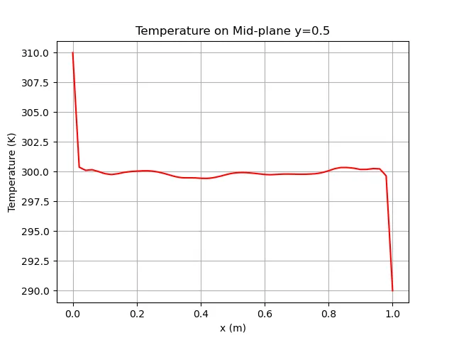
- Thermal Boundary Layers: Because the convective forces are so strong (), heat will not diffuse evenly across the room. Instead, extreme temperature gradients will be confined to very thin boundary layers right next to the hot and cold walls.
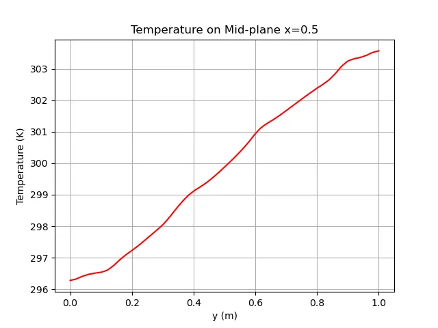
- Core Stratification: The center of the cavity will be mostly stagnant and exhibit thermal stratification—meaning the temperature will be relatively uniform horizontally, but will gradually increase from the bottom of the cavity to the top.
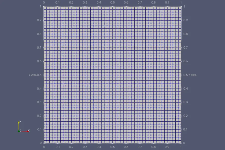
2. Launching the Simulation
We have configured system/controlDict to run buoyantBoussinesqSimpleFoam for 2000 iterations. Because this is a steady-state solver (SIMPLE algorithm), “time” actually represents iteration steps.
To execute the run neatly, we use our automated script:
./runCase.shThis script will:
- Generate the hexahedral mesh.
- Launch the solver in the background.
- Automatically execute our Python validation and PyVista visualization scripts once it finishes.
3. Monitoring Convergence
As the solver marches towards 5,000 iterations, it calculates the residuals for Pressure (p_rgh), Velocity (U), and Temperature (T).
Because we are using a first-order upwind scheme (bounded Gauss upwind in fvSchemes) on a coarse mesh, the solver benefits from high numerical diffusion. This artificial “thickness” stabilizes the highly buoyant flow, allowing the residuals to drop smoothly and plateau. In a fully turbulent high-Ra flow like this, achieving machine-zero residuals is rarely possible on a coarse mesh; instead, we look for the residuals to flatten out, indicating a pseudo-steady state has been reached.
4. Analyzing the Results
Once the simulation completes, we expect the visual contours to exactly match our physical intuition.
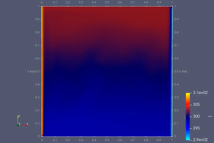
In the temperature contour, look for the sharp red and blue zones hugging the vertical walls. This confirms the presence of thin thermal boundary layers. Notice how the top of the cavity is significantly warmer than the bottom, perfectly illustrating thermal stratification.
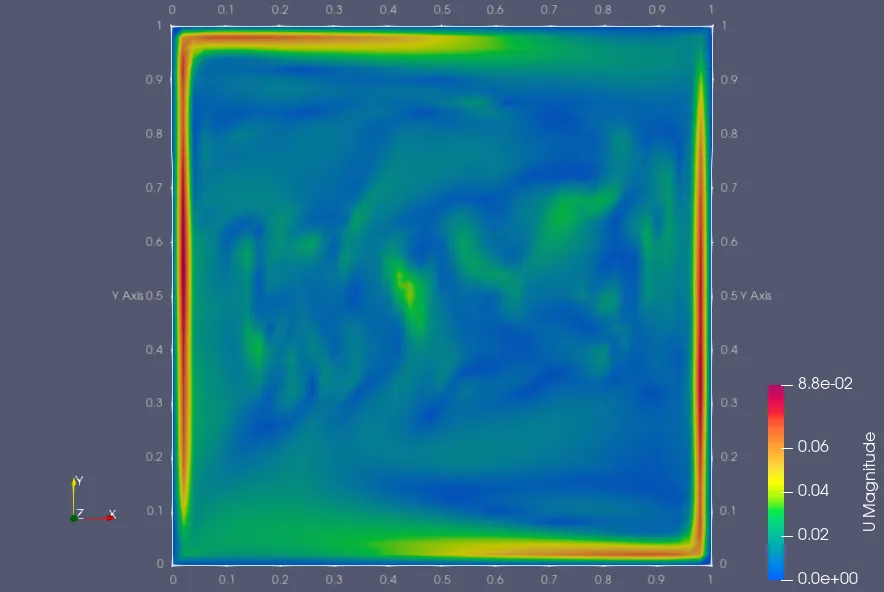
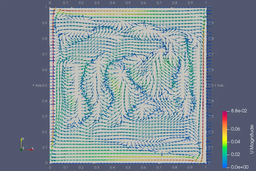
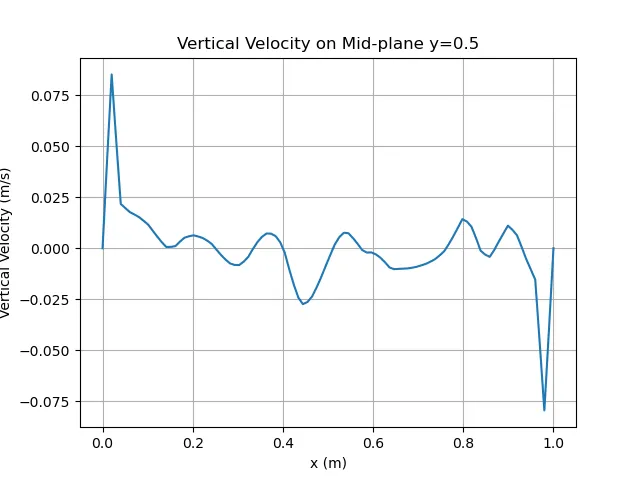
In the velocity fields, the streamlines will reveal the massive clockwise vortex. The highest velocities will be concentrated tightly against the walls where the buoyancy driving force is maximized, while the core remains relatively slow-moving.
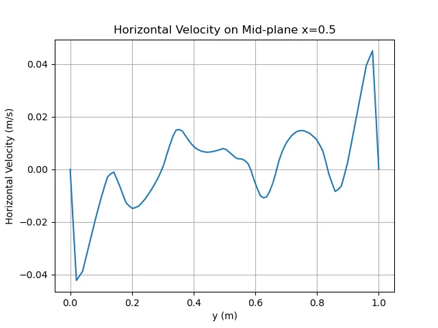
To further validate our results quantitatively, we extract data along the horizontal and vertical mid-planes:
Next Steps
Running the case and getting a pretty picture is only half the battle. While our coarse mesh provides a fantastic qualitative understanding of the convection loop, the heavy numerical diffusion from the first-order schemes means our quantitative data (like the Nusselt number) is likely inaccurate for such a high Rayleigh number.
In future modules, we will perform a Grid Independence Study and upgrade to Second-Order Schemes to capture the true, mathematically rigorous physics!
Related Projects
Part 4: Exploring Turbulent Natural Convection
Transitioning to turbulence in the Differentially Heated Cavity: Exploring k-omega SST for high Rayleigh numbers.
Part 2: OpenFOAM Setup Guide
A comprehensive educational guide to setting up, configuring, and running your first OpenFOAM simulation using the Differentially Heated Cavity.