Part 7: Rayleigh-Number Sweep: Validating a Differentially Heated Cavity in OpenFOAM
A reproducible four-case study of laminar natural convection from Ra = 10^3 to 10^6, compared with the De Vahl Davis benchmark and interpreted with explicit numerical and sampling limitations.
A beginner’s guide to the four-case benchmark
The differentially heated cavity is a useful first thermal-CFD validation problem: a square enclosure, two imposed side-wall temperatures, insulated horizontal boundaries, and gravity. The geometry is simple enough to inspect, while the coupled momentum and energy equations produce buoyancy-driven circulation and nonuniform heat transfer.
This article documents the 05_rayleigh_validation_sweep study in this repository. It is both a tutorial in dimensionless setup and a quantitative report of the current calculation. It distinguishes what the data show from what they do not establish.
1. The benchmark question
Can one OpenFOAM setup reproduce canonical heat-transfer and velocity results over several strengths of laminar natural convection?
The reference is De Vahl Davis’s numerical benchmark for air in a square cavity with differentially heated vertical walls [1]. That study reports accurate two-dimensional solutions across . The present work compares four steady OpenFOAM solutions at exactly those Rayleigh numbers. It is a comparison with a published numerical benchmark, not an experimental validation.
2. Geometry, boundary conditions, and assumptions
The cavity has height and width m. Its left wall is held at K; its right wall at K. The top and bottom are adiabatic. All solid walls are no-slip. Gravity points downward, m s.
OpenFOAM represents the two-dimensional region as a 1 m × 1 m × 0.1 m block with one cell through thickness and empty front/back faces. Each sweep case has a uniform hexahedral mesh.
| Boundary | Velocity | Temperature |
|---|---|---|
| Hot side, | No slip | Fixed at 310 K |
| Cold side, | No slip | Fixed at 290 K |
| Top and bottom | No slip | Zero gradient (adiabatic) |
| Front and back | empty | empty |
The fluid is modeled as Newtonian and incompressible. Density variation appears only in the buoyancy term (Boussinesq approximation); all other properties are constant. Radiation, conjugate heat transfer, compressibility, and three-dimensional effects are omitted.
3. Setting Rayleigh and Prandtl numbers
The two parameters governing the benchmark are
The study fixes K, K, K, m s, m, and . To target each , it changes the kinematic viscosity and thermal diffusivity together:
| Case | (m/s) | (m/s) | |
|---|---|---|---|
Ra_1e3 | |||
Ra_1e4 | |||
Ra_1e5 | |||
Ra_1e6 |
This is a dimensionless benchmark setup: varying effective transport properties is a practical way to change while retaining the geometry and . It should not be mistaken for changing the temperature of a real air-filled device while holding all physical properties fixed.
4. Solver and discretization
All four simulations use buoyantBoussinesqSimpleFoam, a steady incompressible Boussinesq solver, with SIMPLE pressure-velocity coupling. The mesh and schemes are held constant across the sweep. In system/fvSchemes:
div(phi,U)anddiv(phi,T)usebounded Gauss upwind(first-order upwind convection);- gradients use
Gauss linear; - Laplacians use
Gauss linear corrected.
The convective discretization is not second-order linear upwind. Upwind schemes can be robust but add numerical diffusion, which is relevant when interpreting wall gradients and high- boundary layers. The case dictionaries and run scripts are the authoritative configuration.
5. Quantities extracted
The dimensionless velocity components use thermal-diffusion velocity :
The post-processor samples 200 points on the vertical mid-plane and horizontal mid-plane . It reports the positive horizontal-velocity peak on the vertical mid-plane and the positive vertical-velocity peak on the horizontal mid-plane, along with their coordinates. Reporting the positive branch matters: the return-flow peak has nearly equal magnitude at the opposite side of the cavity, but a different coordinate.
For heat transfer, temperature is sampled at m, the first cell-center distance from the hot wall in the uniform mesh. The local wall Nusselt estimate is
This is a near-wall finite-difference estimate and an arithmetic line-sample mean. It is not a direct integration of the OpenFOAM boundary-face heat flux. A wall-gradient post-processing method and a mesh refinement would be preferable for a formal heat-flux uncertainty assessment.
6. Benchmark comparison
The values below compare the sampled OpenFOAM outputs with De Vahl Davis [1]. Relative error is . Velocities are dimensionless as defined above.
| Quantity | OpenFOAM | De Vahl Davis | Error | CFD peak coordinate (reference coordinate) | |
|---|---|---|---|---|---|
| 1.072 | 1.118 | 4.13% | Hot wall | ||
| 3.35 | 3.649 | 8.22% | (0.813) | ||
| 3.38 | 3.697 | 8.65% | (0.178) | ||
| 2.326 | 2.243 | 3.71% | Hot wall | ||
| 16.45 | 16.178 | 1.67% | (0.823) | ||
| 19.79 | 19.617 | 0.88% | (0.119) | ||
| 4.586 | 4.519 | 1.47% | Hot wall | ||
| 35.96 | 34.730 | 3.53% | (0.855) | ||
| 68.37 | 68.590 | 0.31% | (0.066) | ||
| 8.975 | 8.800 | 1.99% | Hot wall | ||
| 66.88 | 64.630 | 3.48% | (0.850) | ||
| 217.86 | 219.360 | 0.68% | (0.0379) |
The mean Nusselt errors are 1.47–4.13%; horizontal peak-velocity errors are 1.67–8.22%; vertical peak-velocity errors are 0.31–8.65%. The errors are not uniformly small: at , both velocity peaks differ from the reference by about 8–9%. At and , the vertical peak is much closer (0.31% and 0.68%).
The complete-precision output is stored in 05_rayleigh_validation_sweep/results/benchmark_validation_summary.csv; the project README is here. The benchmark source is cited in full in References.
7. Flow-regime observations
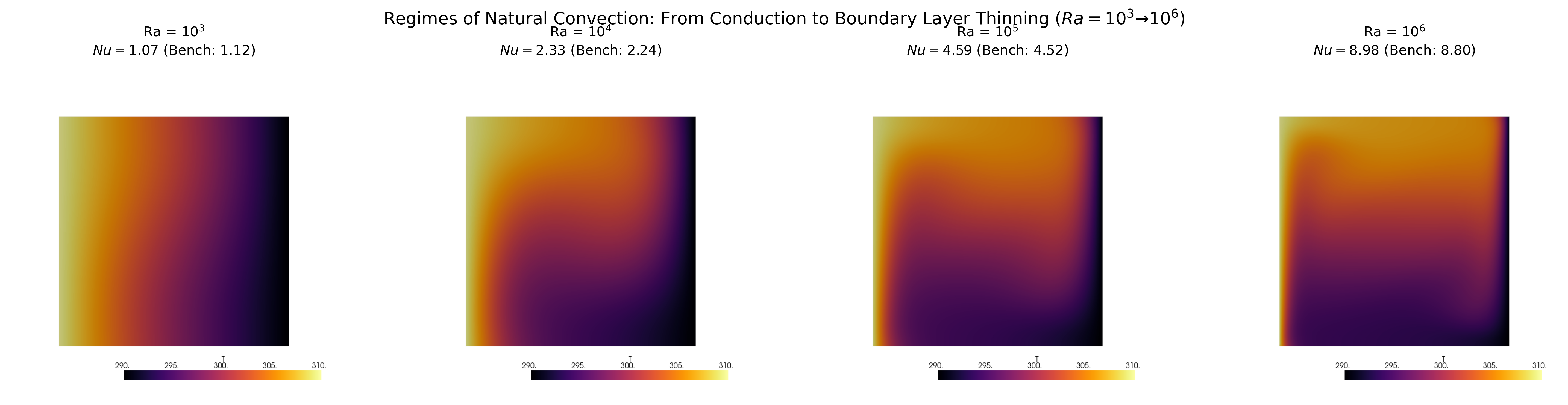
- — conduction-dominated limit. The mean Nusselt estimate is 1.072, close to the pure-conduction value of one. The mid-plane temperature remains close to the linear conduction profile, while buoyancy drives a weak circulation.
- — stronger cavity circulation. The mean Nusselt number rises to 2.326. Temperature contours tilt as fluid transports heat around the cavity.
- — stratified core. The center temperature profile becomes flatter than the conduction line, while stronger gradients persist near the vertical boundaries.
- — wall-dominated transport. The mean Nusselt estimate reaches 8.975. The peak vertical velocity is much larger than at low and occurs closer to the hot wall; the cavity core is comparatively weakly moving and thermally stratified.
These statements describe the computed fields and sampled profiles. They do not imply that the high- boundary layer is fully resolved, nor do the steady laminar solutions establish a physical transition threshold.
8. Trends across the sweep
Heat transfer scaling
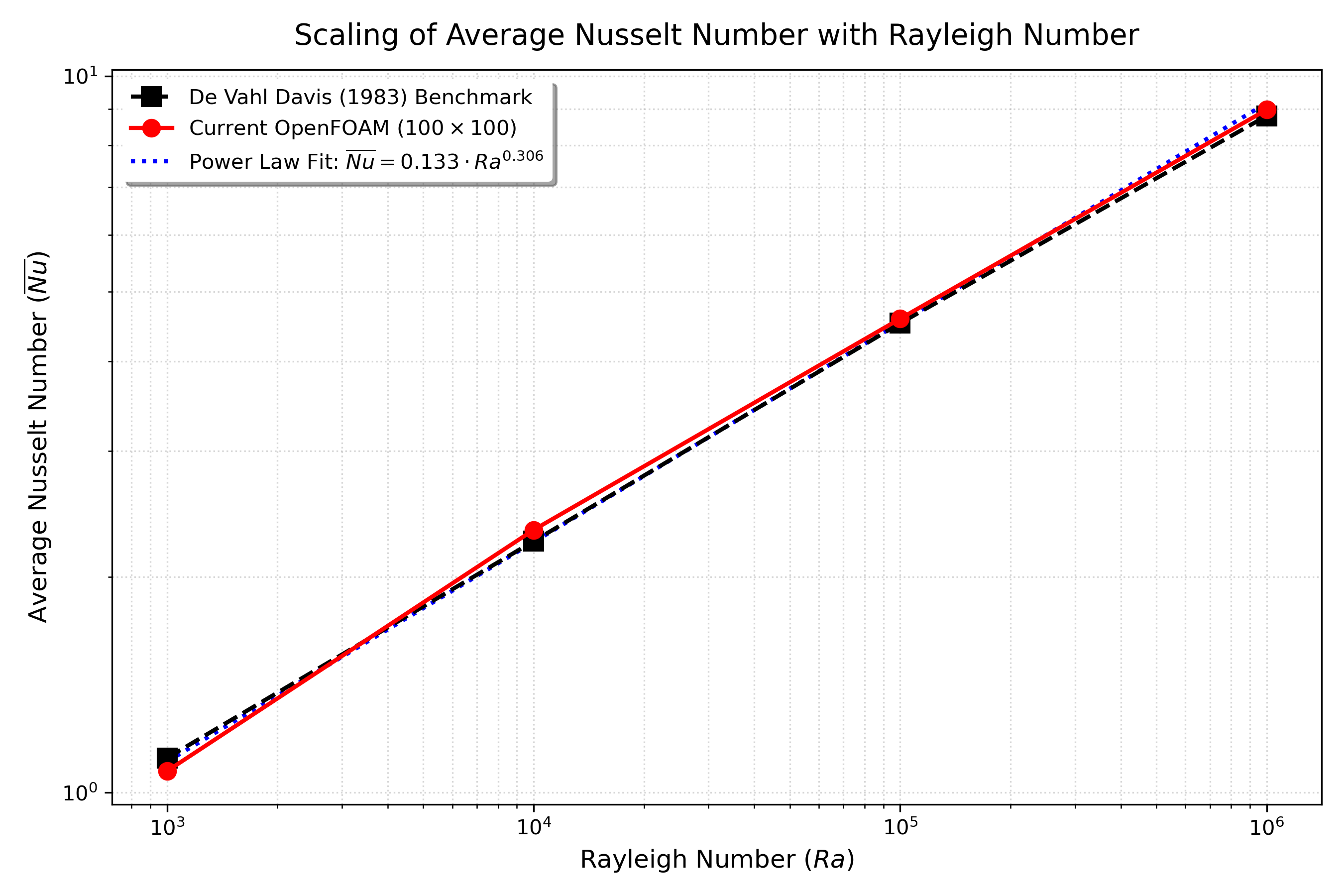
A least-squares fit to the four OpenFOAM data points in log space gives
This exponent is computed from just four discrete values. It summarizes this sweep; it is not a general scaling law and should not be presented as independent validation. A broader parameter range, consistent heat-flux evaluation, and grid refinement are needed before making a stronger scaling claim.
Velocity growth and peak positions
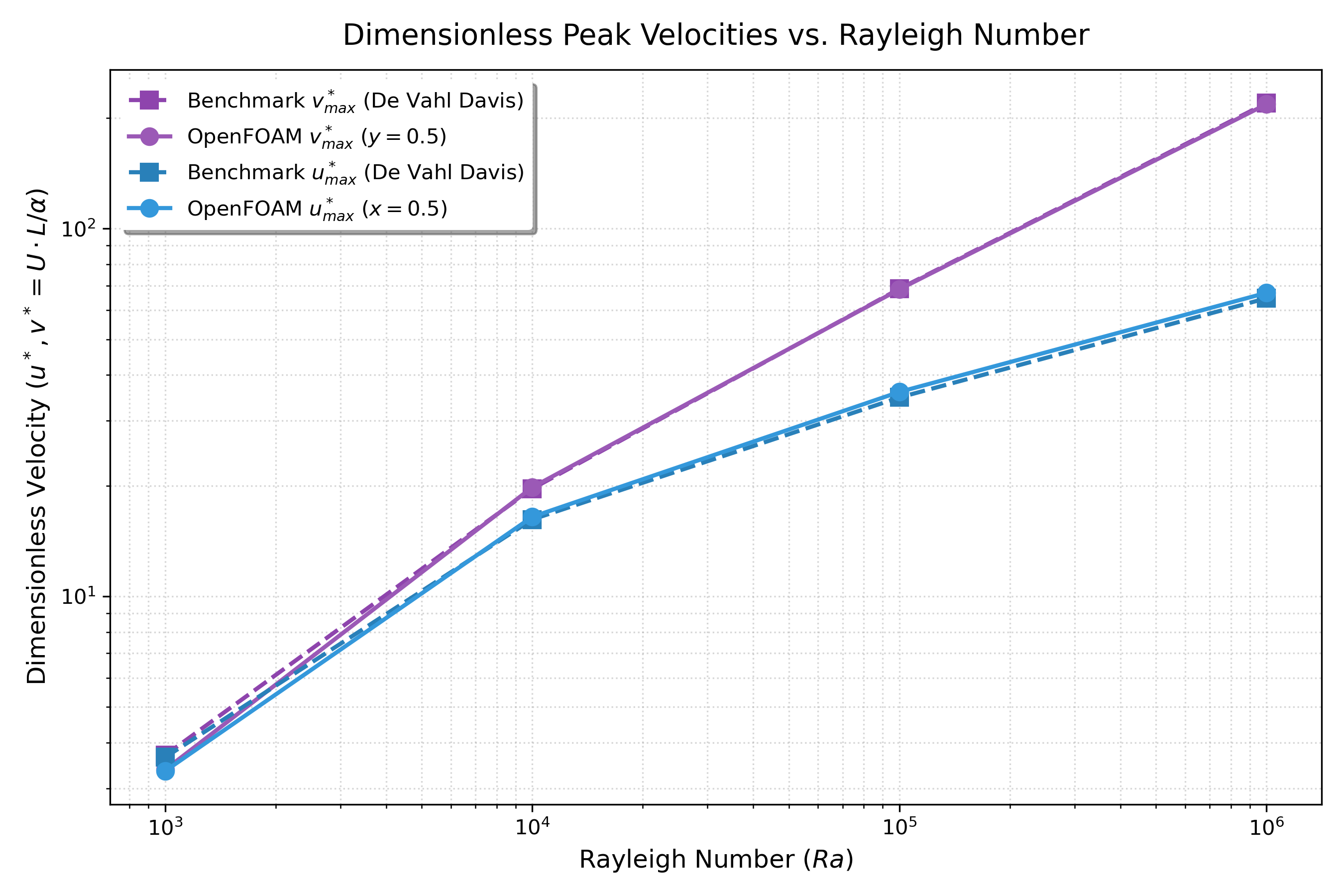
The vertical peak increases from 3.38 to 217.86 (about 64 times), while the positive horizontal peak rises from 3.35 to 66.88 (about 20 times). The four-point log-log fit exponents are approximately 0.597 for and 0.424 for . As with the Nusselt fit, these are descriptive exponents over this limited data set.
The sampled location of the vertical-velocity maximum moves from at to at . This supports the qualitative interpretation of increasing near-wall localization. It is not by itself a direct measurement of boundary-layer thickness: a layer thickness should be defined from a gradient or profile criterion and tested under mesh refinement.
Mid-plane temperature
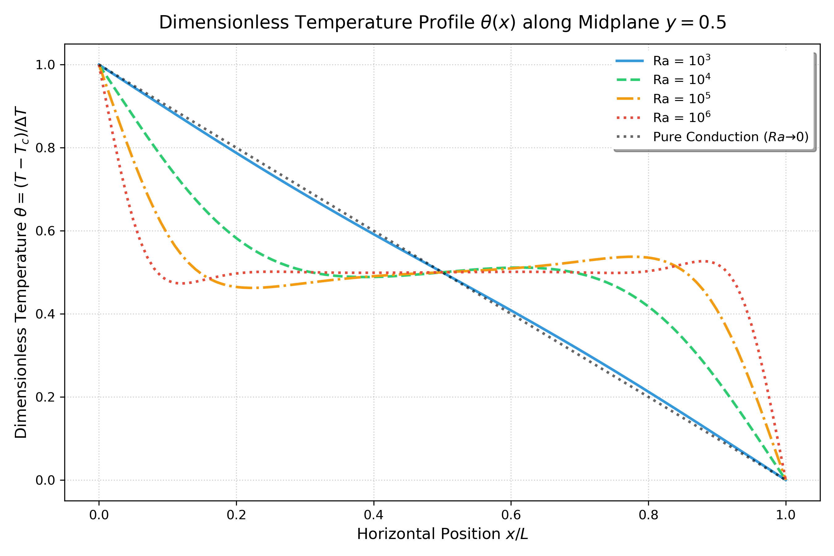
The curve at is close to , where . As increases, convection redistributes heat and the center portion of the curve becomes flatter. The near-wall gradients carry an increasing share of the temperature drop.
Mid-plane vertical and horizontal velocity
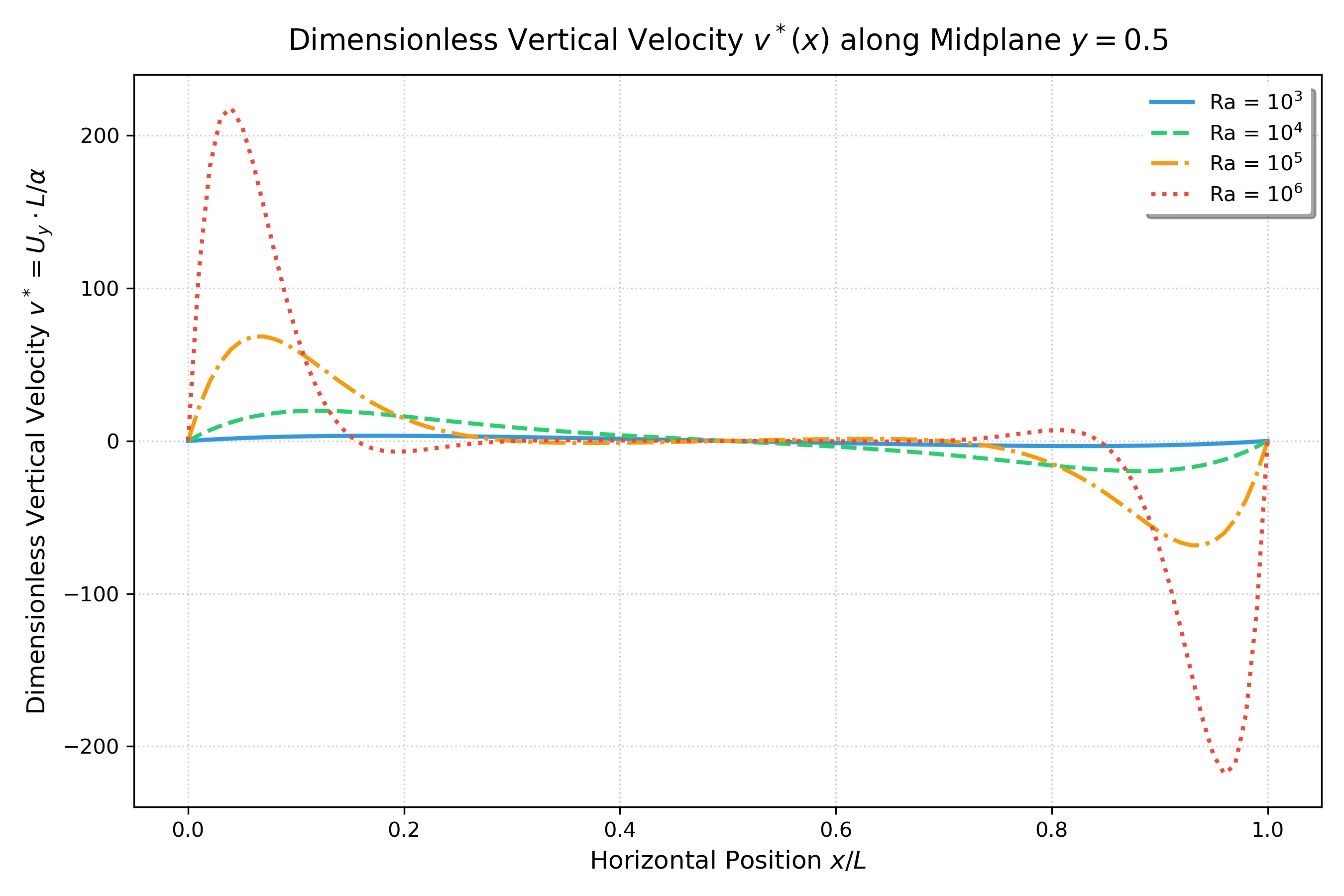
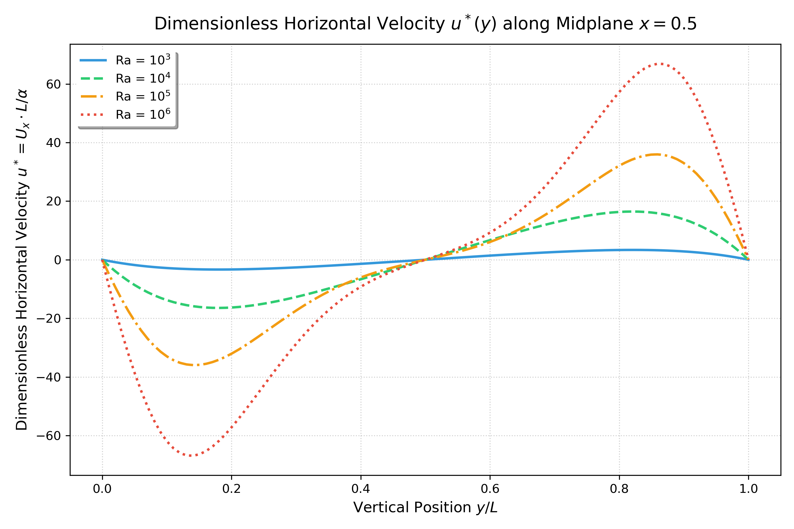
The vertical-velocity profile has a positive hot-side peak and a negative cold-side return branch. On the vertical mid-plane, the horizontal velocity changes sign between the upper and lower parts of the recirculation. The peak magnitudes alone do not capture all of this profile structure, so the plots and raw sample files are useful for learning and independent re-analysis.
Local near-wall Nusselt estimate
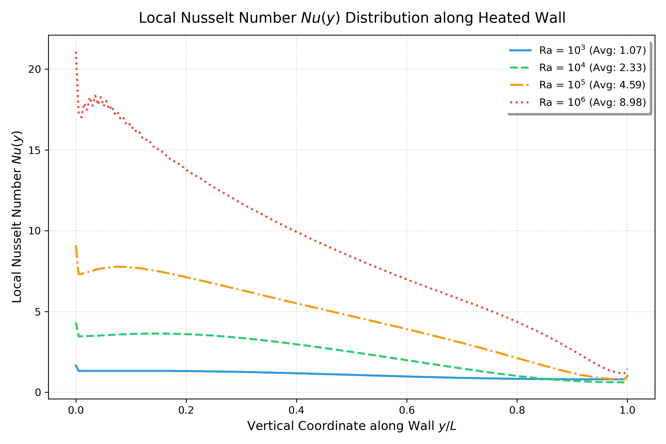
The estimated local Nusselt number becomes more nonuniform with increasing . The profile is relatively flat compared with the stronger spatial variation at higher . Because the line is offset from the wall and the mesh is uniform, the plot is best interpreted as a qualitative profile; do not treat the local extrema as mesh-independent wall heat flux.
9. Reproduce the calculation
Install OpenFOAM.com v2512 or a compatible release with blockMesh and buoyantBoussinesqSimpleFoam. The post-processing script requires Python 3 and NumPy, pandas, Matplotlib, and PyVista.
cd 05_rayleigh_validation_sweep
./Allrun
The runner builds and solves each of the four cases before generating the comparison table and figures. Each case writes log.blockMesh and log.foam; sampled CSV files are under cases/Ra_*/postProcessing/. To process existing solutions without rerunning the solvers:
python3 scripts/postprocess_benchmark_sweep.pyThe runner is designed to stop when a case fails; the post-processor also reports missing sample data rather than producing a success-shaped partial summary.
10. What this study does not establish
- No sweep-specific grid uncertainty: all four Rayleigh numbers use one 100 × 100 in-plane mesh. The separate grid study is a different operating condition and cannot quantify sweep error.
- No formal solver convergence report: the summary records final sampled fields, not a residual-based or monitored-quantity convergence history.
- Numerical diffusion: first-order bounded upwind convection can smooth steep boundary-layer profiles.
- Approximate wall gradient: the hot-wall flux uses a temperature sample at m and a finite difference. Mesh refinement and a boundary-face gradient integration are needed for stronger heat-transfer claims.
- Discrete peak locations: 200-point line samples limit coordinate precision; a few thousandths of is not a meaningful exact difference.
- Steady laminar assumption: all four cases use a steady laminar solver, including . This sweep does not demonstrate whether the physical flow becomes unsteady or turbulent.
- Idealized physics: constant properties, Boussinesq density variation, two-dimensional geometry, and no radiation or conjugate conduction are assumptions.
For future studies, use a scheme/grid refinement, monitor heat flux and residuals to steady convergence, compare wall-gradient and profile-based quantities, and report uncertainties separately from benchmark differences.
References
- De Vahl Davis, G. (1983). “Natural convection of air in a square cavity: A bench mark numerical solution.” International Journal for Numerical Methods in Fluids, 3(3), 249–264. https://doi.org/10.1002/fld.1650030305.
- OpenCFD Ltd. OpenFOAM v2512 Documentation. https://doc.openfoam.com/.
- Celik, I. B., Ghia, U., Roache, P. J., Freitas, C. J., Coleman, H., & Raad, P. E. (2008). “Procedure for estimation and reporting of uncertainty due to discretization in CFD applications.” Journal of Fluids Engineering, 130(7), 078001. https://doi.org/10.1115/1.2960953.
Related Projects
Part 6: Mesh Verification & Grid Convergence Index (GCI)
Quantifying numerical discretization error and establishing mesh independence in the Differentially Heated Cavity using Richardson Extrapolation and the ASME V&V 20 Standard.
Part 4: Exploring Turbulent Natural Convection
Transitioning to turbulence in the Differentially Heated Cavity: Exploring k-omega SST for high Rayleigh numbers.