Part 4: Exploring Turbulent Natural Convection
Transitioning to turbulence in the Differentially Heated Cavity: Exploring k-omega SST for high Rayleigh numbers.
Author: Martin Mathew | Date: 2026-10-08 | Category: Thermal CFD Tutorial
1. The Transition to Turbulence
In our previous article, we established the baseline for a 2D Differentially Heated Cavity (DHC). While that case provides an excellent foundation, the Rayleigh number () we computed reached . In natural convection, transition to turbulence typically occurs when exceeds or . This means our baseline case was already pushing the boundaries of the laminar regime!
As the temperature difference () increases or the physical size of the cavity expands, buoyancy forces begin to dominate viscous dampening. The flow transitions from smooth, predictable laminar streamlines to chaotic, eddy-rich turbulent flow.
In a Differentially Heated Cavity, this transition is highly localized. It usually begins in the boundary layers along the vertical heated and cooled walls, while the core of the cavity might remain relatively calm or become highly stratified. Capturing this physics requires moving beyond a simple laminar assumption.
2. Turbulence Modeling for Buoyancy-Driven Flows
Direct Numerical Simulation (DNS) resolves all turbulent scales but is computationally prohibitive for engineering applications. Instead, we rely on Reynolds-Averaged Navier-Stokes (RANS) models.
For thermal boundary layers, the SST (Shear Stress Transport) model is widely considered the industry standard. It excellently resolves the near-wall physics (where the thermal gradients are steepest) using the formulation, while switching to a formulation in the free stream to avoid sensitivity to freestream turbulence.
3. Meshing: The Importance of Near-Wall Resolution
Turbulence models, especially those resolving the boundary layer like SST, are highly sensitive to mesh resolution. The viscous sublayer must be accurately captured. In our updated setup, we refine the mesh from 50x50 to 100x100 to ensure there are enough cells clustered near the walls.
For highly accurate heat flux (Nusselt number) calculations, maintaining a wall distance () of approximately 1 is crucial.
4. Configuring OpenFOAM for Turbulence
To transition our case, we made several modifications:
constant/turbulenceProperties: We switchedsimulationTypefromlaminartoRASand specified thekOmegaSSTmodel.system/fvSchemesandfvSolution: We added numerical schemes and solver settings for the new turbulent quantities: turbulent kinetic energy () and specific dissipation rate (). Crucially, we included thewallDistscheme, which SST relies on for its blending functions.- Boundary Conditions (
0/directory): We introduced appropriate wall functions for:- :
kqRWallFunction - :
omegaWallFunction - (turbulent kinematic viscosity):
nutkWallFunction - (turbulent thermal diffusivity):
alphatJayatillekeWallFunction(designed specifically to capture thermal boundary layers by utilizing the turbulent Prandtl number, ).
- :
5. Results and Physical Insights
With the simulation complete, let’s look at the extracted data from the new case_turbulent!
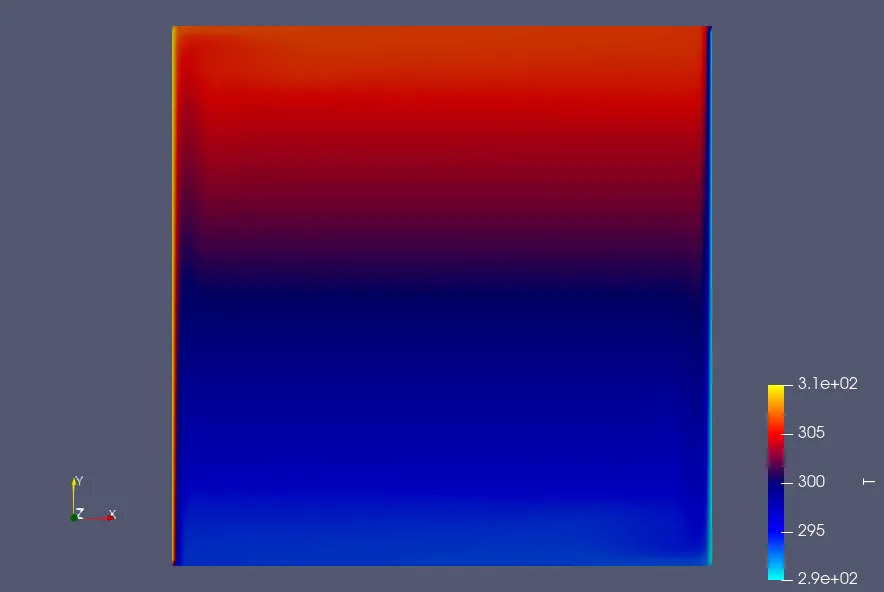
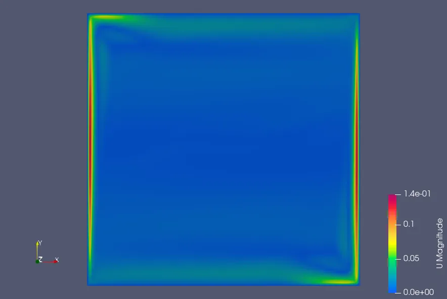
- Velocity Profiles: The peak vertical velocity () along the mid-plane increased substantially from m/s (in our baseline laminar assumption) to m/s with the SST model. The near-wall velocity peaks are sharper and closer to the walls, which is characteristic of a turbulent boundary layer.
- Core Stratification: The horizontal velocity () across the mid-plane dropped from m/s to m/s. This indicates that the strong recirculating structures in the center of the cavity have been dampened by turbulent mixing, leading to a much flatter and more stratified core region.
- Temperature Profiles: The maximum temperature measured just outside the viscous sublayer () remains around K. The turbulent mixing drastically flattens the temperature gradient in the center of the cavity, effectively acting as an insulator, while creating extremely steep temperature gradients directly adjacent to the hot and cold walls.
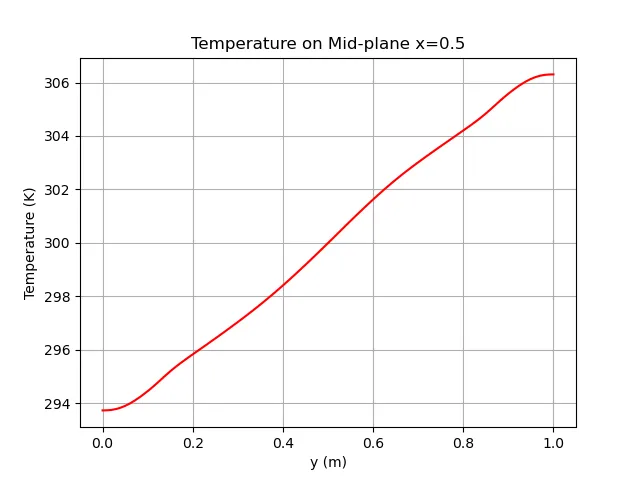
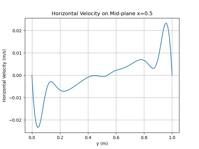
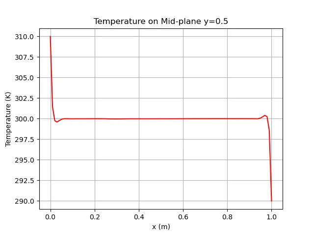
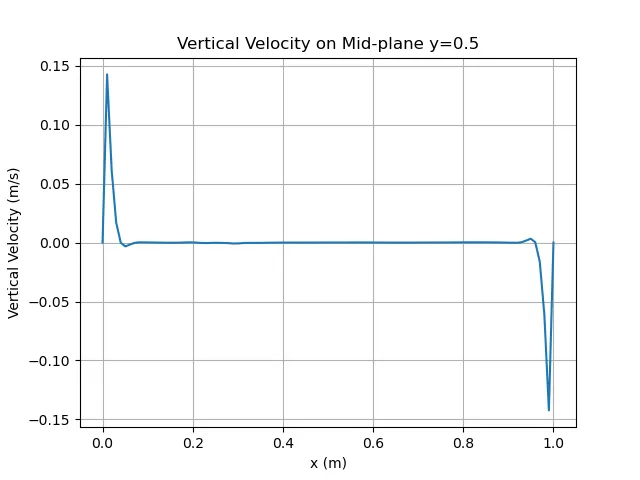
By successfully moving to a turbulent solver, we have captured a far more realistic flow state for high Rayleigh numbers (). The SST model accurately predicts the strong boundary layer jets and the quiescent, stratified core—essential phenomena for industrial natural convection problems!
Related Projects
Part 3: Running the 1x1 Case
Execution and analysis of the 1x1 Differentially Heated Cavity case in OpenFOAM, exploring steady-state natural convection.
Part 7: Rayleigh-Number Sweep: Validating a Differentially Heated Cavity in OpenFOAM
A reproducible four-case study of laminar natural convection from Ra = 10^3 to 10^6, compared with the De Vahl Davis benchmark and interpreted with explicit numerical and sampling limitations.