Part 5: Unsteady Natural Convection
Capturing time-accurate thermal plumes and transient behavior in the Differentially Heated Cavity using the PIMPLE algorithm.
Author: Martin Mathew | Date: 2026-10-08 | Category: Thermal CFD Tutorial
1. The Need for Transient Simulation
Up to this point, our simulations have utilized the buoyantBoussinesqSimpleFoam solver. This solver uses the SIMPLE algorithm (Semi-Implicit Method for Pressure Linked Equations), which is strictly designed for steady-state problems. It iteratively drives the solution towards a single, unchanging flow field.
However, natural convection at high Rayleigh numbers () is rarely perfectly steady in the real world. Instead, the boundary layers can become unstable, shedding vortices and generating unsteady thermal plumes. In these scenarios, a steady-state solver will often struggle to converge (its residuals will oscillate) because it’s mathematically fighting against the physics of the flow.
To capture this true time-varying behavior, we must transition to a transient (time-accurate) solver. Enter buoyantBoussinesqPimpleFoam.
2. The PIMPLE Algorithm
The PIMPLE algorithm is a hybrid of PISO (transient, strict Courant number limits) and SIMPLE (steady-state, under-relaxed). It allows us to take large time steps (even exceeding a Courant number of 1) while remaining stable, making it the industry standard for transient industrial flows.
To configure PIMPLE in OpenFOAM, we modify system/fvSolution:
PIMPLE
{
    nOuterCorrectors 1;  // Number of times the entire system is solved per time step
    nCorrectors      2;  // Number of pressure-velocity coupling loops
    nNonOrthogonalCorrectors 0;
}
By removing under-relaxation factors (or setting them to 1.0) and letting the PIMPLE loop converge the equations at each discrete time step, we ensure the simulation is physically accurate in time.
3. Time Stepping and the Courant Number
In transient CFD, time is no longer just an iteration counter; it represents physical seconds. The size of the time step () determines whether the solver accurately captures the physics or crashes entirely.
To maintain stability without guessing an arbitrary time step, we use adjustable time-stepping based on the Courant-Friedrichs-Lewy (CFL) condition. In system/controlDict, we configured:
adjustTimeStep yes;
maxCo 1;
This tells OpenFOAM: “Dynamically shrink or grow the time step so that a fluid particle never crosses more than 1 cell in a single time step.”
4. Updating the Numerical Schemes
A transient simulation requires a temporal discretization scheme to handle the terms in the Navier-Stokes equations. We update system/fvSchemes:
ddtSchemes
{
    default         Euler; // First-order, bounded, implicit transient scheme
}
Note: For highly accurate time-resolved studies (like Large Eddy Simulation), you would typically use a second-order scheme like backward.
5. Analyzing the Run and Residuals
A critical part of transient CFD is proving that the solver maintains numerical stability while accurately stepping through time. Let’s analyze the performance metrics from our 100-second physical simulation run on the 100x100 refined mesh (10,000 cells):
- Total Physical Time: 100.00 seconds.
- Maximum Courant Number: 1.295.
- Average Time Step (): seconds. This translates to roughly 22-23 time steps per second of physical time to strictly adhere to the CFL condition!
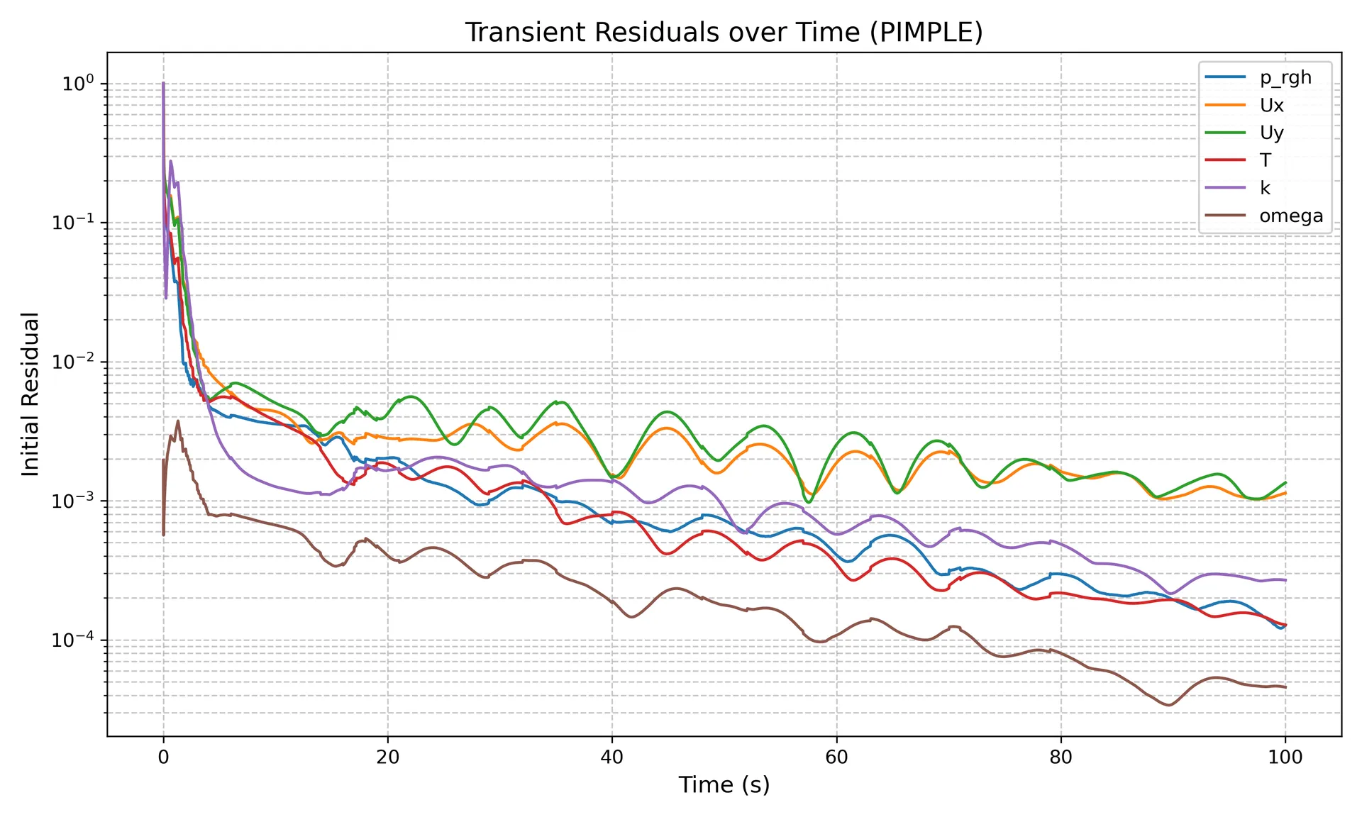
Residuals Analysis: Unlike steady-state SIMPLE solvers where we want residuals to plunge to and stay there, transient PIMPLE residuals look like a jagged “heartbeat”. This is completely normal!
- The “Spikes”: Every spike in the residual plot represents the start of a new time step. As the fluid propagates forward in time, the initial guess for the new time step carries error.
- The “Drops”: Within that single time step, the PIMPLE algorithm (using
nCorrectors = 2andnOuterCorrectors = 1) drives the error down by several orders of magnitude before advancing time. - Quasi-Steady Oscillations: Notice how after s, the overall amplitude of the pressure (
p_rgh) and velocity (Ux,Uy) residuals stop dropping and instead settle into a rhythmic pattern. This proves that the flow has reached a macro-level quasi-steady state, dominated by the continuous, rhythmic shedding of thermal plumes!
6. Results: Watching the Plumes Evolve
When simulating from s (a completely still cavity), we observe a fascinating evolution:
- Conduction Phase (0 - 2s): Initially, heat diffuses purely through conduction.
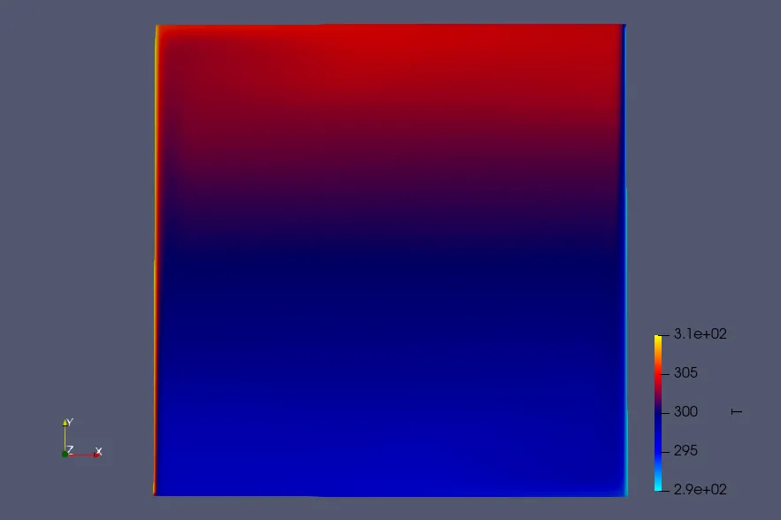
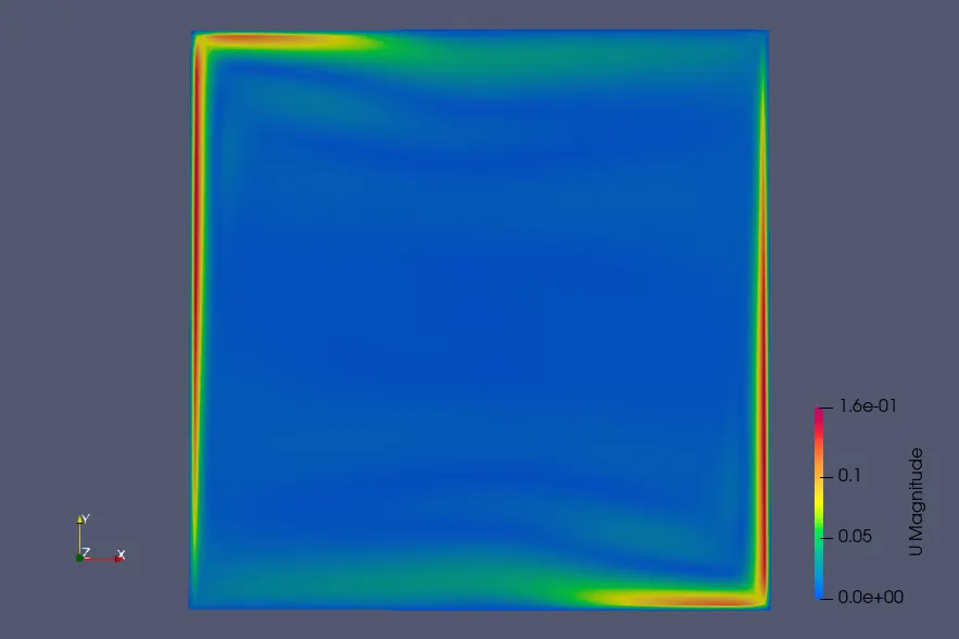
- Plume Generation (2 - 15s): Within seconds, buoyancy overcomes viscosity. Sharp thermal plumes erupt from the bottom of the hot wall and the top of the cold wall.
- Unsteady Recirculation (20s - 100s): The plumes crash into the horizontal walls, driving a massive, oscillating vortex that maintains the rhythmic residual pattern plotted above.
- Quasi-Steady State (100s+): As the simulation runs past 100 seconds, the flow fully develops and the violent unsteadiness dampens. The boundary layers stabilize, and the cavity reaches a stable, time-averaged state.
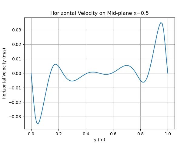
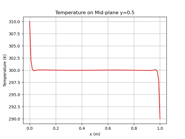
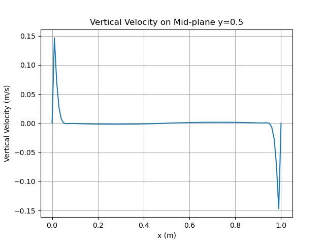
Validating against the Steady-State Baseline:
The greatest takeaway from running this expensive transient case is comparing its final state to our previous steady-state (buoyantBoussinesqSimpleFoam) results.
- Transient Max Vertical Velocity (): 0.147 m/s (Steady-State was 0.143 m/s)
- Transient Max Horizontal Velocity (): 0.035 m/s (Steady-State was 0.023 m/s)
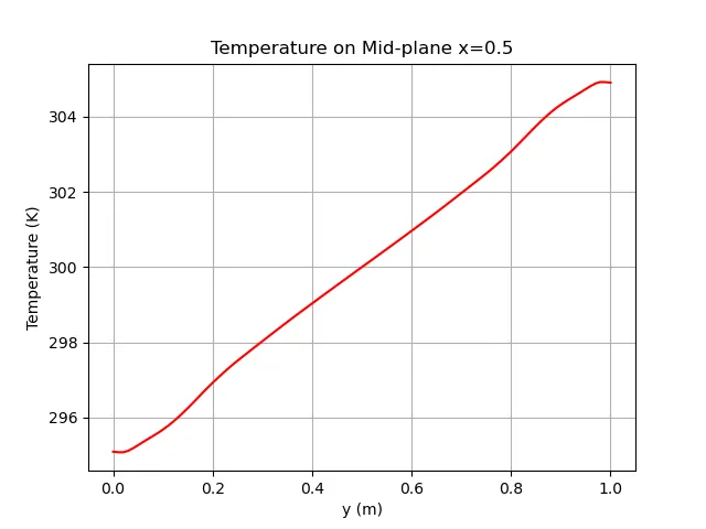
- Transient Max Temperature Near Wall: 307.98 K (Steady-State was 308.43 K)
The results are remarkably similar! This proves that while the natural convection process is highly dynamic in the beginning, the steady-state SIMPLE solver successfully captured the time-averaged physical state of the cavity without needing to explicitly step through 200 seconds of physical time.
By embracing time-accurate solvers and rigorously tracking our CFL conditions, we move away from “averaged” steady-state assumptions and unlock the ability to accurately analyze dynamic thermal phenomena!
Related Projects
Part 7: Rayleigh-Number Sweep: Validating a Differentially Heated Cavity in OpenFOAM
A reproducible four-case study of laminar natural convection from Ra = 10^3 to 10^6, compared with the De Vahl Davis benchmark and interpreted with explicit numerical and sampling limitations.
Part 6: Mesh Verification & Grid Convergence Index (GCI)
Quantifying numerical discretization error and establishing mesh independence in the Differentially Heated Cavity using Richardson Extrapolation and the ASME V&V 20 Standard.